Research on Virtual Track Train Path-Tracking Control Based on Improved MPC and Hierarchical Framework: A Reconfigurable Approach

Abstract

The virtual track train (VTT) is a new urban public transportation system that adopts all-axle steering and distributed drive. The Super autonomous Rail rapid Transit (SRT), as one of them, adopts a four-module six-axle structure. In response to its crucial problem, its path tracking, this article proposes a reconfigurable dynamic modeling method, which has two parts: a multi-body dynamics model with generalized forces at each module’s center of gravity (CG) as the input, and the CG generalized force model, which expresses the CG generalized forces generated by the wheel control inputs. Then, a path-tracking strategy is proposed based on the improved MPC and hierarchical framework. Firstly, the CG generalized forces of each module required for path tracking were calculated, and then the CG generalized force redistribution was performed and the “virtual axle” method was proposed. Finally, the wheel state of each module was allocated. This strategy reduces the complexity of each layer of the controller and it solves the problem of insufficient actuators in the middle two modules of the SRT. Finally, through a hardware-in-the-loop (HIL) real-time simulation and comparison with different control strategies, the control strategy’s effectiveness, adaptability, and robustness were verified.

1. Introduction

Urban population growth and car ownership have put enormous pressure on public transport [1]. Although it can be alleviated by subways, trams, and other ways, there are shortcomings such as high construction costs, long construction periods, and high maintenance costs [2]. To overcome the above problems, a kind of public transportation system called the virtual track train (VTT) has been developed rapidly in recent years.

The VTT is a multi-articulated public transportation system using a rail transit management mode. The so-called “virtual track” differs from traditional rail systems’ track. It does not have a strong constraint between the track and the vehicle but is composed of ground markers or magnetic spikes and is a digital track. The VTT adopts rubber tire running gears and uses environmental perception technology to recognize the virtual track and environment. Then, path-tracking control technology is used to control the wheel steering angles of each axle and the driving torque of the driving wheels, allowing the vehicle to autonomously track the target path and speed with high accuracy. Compared with traditional rail transit systems, the construction costs, construction cycle, and maintenance costs of the VTT can be significantly reduced [2,3]. Compared with bus rapid transit (BRT), the VTT has some advantages. The longer body can carry more passengers, and its capacity is equivalent to trams. The all-axle steering and distributed drive technology make it more flexible and have a smaller sweep width, which can pass through curves with smaller radii. The VTT has received widespread attention recently, and multiple operational lines have been built.

At present, there are mainly three types of VTTs in commercial operation: Super autonomous Rail rapid Transit (SRT) released by CRRC Zhuzhou Locomotive Co., Ltd. in Zhuzhou of China, Automatic Rail rapid Transit (ART) released by the CRRC Zhuzhou Institute in Zhuzhou of China, and Digital Rail guided Train (DRT) released by CRRC Nanjing Puzhen Co., Ltd in Nanjing of China. The SRT adopts a four-module marshalling. The first and fourth modules each have two steerable rubber wheel running gears and the middle module has one steerable rubber wheel running gear. The first axle of the first module and the second axle of the fourth car (the first and sixth axles of the entire vehicle) are equipped with drive motors, and adjacent modules are connected through hinge plates. The ART adopts a three-module marshalling. Each module is equipped with two independent steering rubber wheel running gears. The DRT train also has a three-module marshalling, but adjacent modules are connected through articulated double-axle rubber wheel bogies. In addition, there are also some transportation systems with operational characteristics and control methods similar to the VTT, for example, the AutoTram Extra Grand series developed by the Fraunhofer Institute in Germany [4], the Civis optical guided bus developed by Siemens and Iveco, the Phileas guided bus system developed by the VDL Group in the Netherlands [5], and the TEOR system operated commercially in Rouen, the capital of the Normandy, in France [6]. Among them, the SRT has a higher carrying capacity and curve passing flexibility due to its larger number of marshalling, making it more advantageous than other transportation systems.

The path-tracking control technology is the key to the safe and stable operation of the VTT along the target path with minimal error. Refs. [7,8,9,10,11] introduce some control strategies for single articulated vehicles with tractor–trailer combinations to ensure mobility at low speed and medium- and high-speed stability. These methods use the articulated point of the tractor as the following point of the trailer for tracking control based on the vehicle kinematics model. Oreh [12] adopted a control method based on the ideal articulation angle, which controls the steering angle of each wheel to ensure that the articulation angle is at the optimal value to eliminate the tracking error. Refs. [7,13,14] calculate the target state of the vehicle based on the established kinematics model and then propose a specific control law for the wheel steering angle. Kolb [15] also achieved path tracking under reversing conditions by accurately linearizing the nonlinear model of the vehicle. In order to improve passenger capacity, driving capacity, and operational quality, multi-module marshalling, all-axle steering, and distributed drive are the inevitable directions for the development of the VTT. However, the above research focuses on the tractor–trailer configuration, which is somewhat different from the multi-articulated and multi-actuator system of the VTT.

The research on multi-articulated systems can be traced early [16], and is similar to the active trailer steering (ATS) problem in a wheeled mobile robot (WMR) [17,18]. Bolzern [19,20] considered the tracking problem of a vehicle composed of a single tractor and an N-1 trailer equipped with off-axle hinges. A vehicle input–output feedback linearization model was established and a zero dynamic analysis of the system was conducted. Finally, the path-tracking control was completed by assigning closed-loop poles to the linearized system. Astolfi [21] adopted Lyapunov-based methods to achieve asymptotic stability control of articulated vehicles’ forward and backward motion. Refs. [22,23] adopt a method based on extended Ackermann steering, which determines the instantaneous center of rotation based on the steering angle of the vehicle’s first axle. By controlling the steering angle of other wheels to make the instantaneous centers of each wheel the same, all wheels can track the midpoint of the first axle. Sebastian Wagner and Bernard Baeker [24] researched dynamics-based tracking methods. The article first establishes the dynamic and tire models of multi-articulated vehicles using the principle of virtual displacement and virtual work and proposes a feedforward and feedback control strategy. The lateral force at the axle required for path tracking is calculated based on tracking error, and then the wheel steering angle is obtained through reverse-solving the tire model. De Bruin and Oreh [25,26] proposed a full-state tracking control algorithm based on the vehicle dynamics model by taking all degrees of freedom (DOFs) as the vehicle state and taking the rotation angles of each axle and the driving torque of each wheel as control inputs. Maciej Marcin Michalek [27] proposed a universal tracking control method for N-unit wheeled robots. Moreover, thanks to the proposed cascaded control modules, the controller can quickly expand based on the number of marshalling, and the effectiveness of the control method was verified through a theoretical model. Leng [28] proposed a scalable cascade modular path following a control strategy for the gantry virtual track train (G-VTT) based on a preview and tracking controller focusing on the lateral control for low-speed turning maneuvers, and the lag time was considered. Feng [29] introduced the path-tracking control of the ART. Firstly, the tracking error was calculated through the image processing method, and two different control methods for the first module were proposed based on preview PID and Model Predictive Control (MPC). Then, the steering angle of each subsequent wheel was calculated based on the extended Ackermann method. Furthermore, a first-order delay was added to meet the different instantaneous rotation centers when the vehicle passes through the transition curve.

Due to the characteristics of multi-module marshalling, all-axle steering, and distributed drive, the number of control inputs of the VTT is much greater than its DOFs, which makes the path-tracking problem difficult. Moreover, unreasonable control strategies can worsen hinge and tire force [30,31]. In addition, the current control strategy based on the kinematics model ignores the tire sideslip, resulting in low tracking accuracy at medium and high speeds. At the same time, the end-to-end control strategy based on the dynamics model is too complex, which is not conducive to the real-time deployment of the controller [32]. In addition, the VTT has multiple types of structure, and the current control strategy is not universal.

Under these challenges, the main contribution as well as the core goal of this paper is to develop a reconfigurable control strategy that could apply to any configurations and drive modes of VTTs for dynamics path-tracking control, meanwhile reducing the hinge forces and tire sideslip. A simple and elementary control strategy has been reported in [33]; nevertheless, it just referred to the all-wheel-drive vehicles with two axles per module and used a hypothetical theoretical model without specified vehicle parameters. Differentiating from the previous work, this paper introduces an extended modeling process, a newly designed and completed controller, and a very different vehicle case study. Considering the different number of modules, each module may have a different number of axles, and only some axles have driving capacity, for example, the four-module six-axle SRT; leveraging this methodology, one could just set the defined “Boolean matrix” based on the vehicle configuration and perform minor tuning, and a new dynamics model and controller would be obtained. Moreover, for the structural specificity SRT, in addition to the improved MPC and hierarchical architecture, we proposed CG generalized force redistribution and the “virtual axle” method to avoid significant control errors caused by insufficient actuators in the middle two modules. The vehicle dynamics model of the SRT is established based on the authentic parameters, and the proposed control strategy is verified through a hardware-in-the-loop (HIL) real-time simulation. It is hoped that this approach will provide a new perspective for VTT dynamics control.

The second part of this paper introduces the structure of the SRT and establishes the vehicle dynamics model. The third part proposes and implements a path-tracking control strategy based on an improved MPC algorithm and hierarchical architecture. The effectiveness of the control strategy is verified through an HIL real-time simulation in Section 4. The conclusion is drawn in Section 5.

2. SRT Structure and Dynamics Model

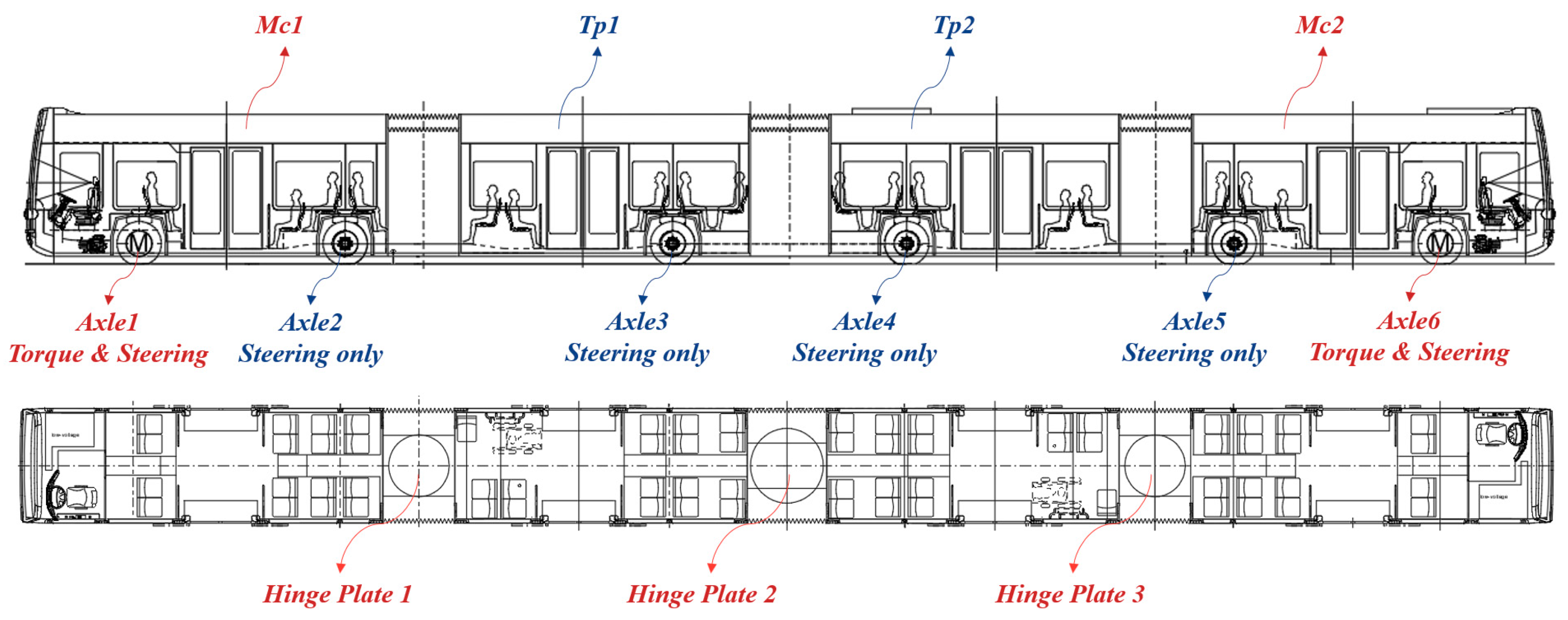
Figure 1 shows the basic structure of the SRT, with a total length of 35 m, a width of 2.55 m, and a floor height of 0.35 m. The SRT adopts a four-module marshalling, with the first and fourth modules being the same structure, equipped with a cab, and each with two rubber wheel running gears that can independently steer. The second and third modules have one steerable rubber wheel running gear. The SRT has six axles: the first and sixth axles are equipped with drive motors to provide torque, while the remaining axles are unpowered. Each module is connected through a hinge plate [34].

When establishing the dynamics model, the following assumptions are made:

Assuming that the vehicle runs on a flat surface, only the movement in the XOY plane and rotation around the Z-axis is considered, ignoring the rolling and vertical movements.

The steering angles of the left and right wheels of the same axle are equal.

The vehicle is considered a multi-rigid body system.

The vehicle dynamics model and CG generalized forces are briefed in [33], but the reconfigurable features were not included. First, a single-module dynamics model is established with the CG generalized and hinge forces as control inputs. The hinge is equivalent to the constraint between adjacent modules. A full-state dynamics model of the entire vehicle is obtained through matrix assembly. Then, the hinge constraint equations are combined to obtain the expression of the hinge force using the vehicle state and CG generalized forces. The dynamics model that can be directly used for model-based control algorithm design is obtained by preserving the DOFs related to path tracking. Finally, the vehicle CG generalized forces can be calculated from the tire force generated by the wheel control input. We newly defined the “Boolean matrix” to determine the availability of axles, namely the axles’ quantity and their ability to provide torques of the wheels. This method can quickly expand and reconstruct the dynamics model for a different number of modules and different configurations of wheels per module.

2.1. Single-Module Dynamics Model

The schematic diagram of the DOFs and forces of the $i^{th}$ module is shown in Figure 2. The longitudinal motion $x^i$, lateral motion $y^i$, and yaw motion ${\psi }^i$ are considered, and the corresponding speeds are represented as $v_x^i$, $v_y^i$, and ${\gamma }^i$, respectively.

For the $i^{th}(i=1,2,3,4)$ module, the dynamics equation with the CG generalized forces and the hinge forces as the input can be written by the Newton–Euler formula:

$$F_x^i+F_{hx,f}^i+F_{hx,r}^i=m^i({\dot{v}}_x^i-{\gamma }^i{\dot{v}}_y^i),$$

(1)

$$F_y^i+F_{hy,f}^i+F_{hy,r}^i=m^i({\dot{v}}_y^i+{\gamma }^i{v}_x^i),$$

(2)

$$M_z^i+l_{f,i}{F}_{hy,f}^i-l_{r,i}{F}_{hy,r}^i+M_{hz,f}^i+M_{hz,r}^i=I_z^i{\dot{\gamma }}^i,$$

(3)

$${\dot{x}}^i=v_x^i,$$

(4)

$${\dot{y}}^i=v_y^i,$$

(5)

$${\dot{\psi }}^i={\gamma }^i,$$

(6)

where the CG generalized forces are $F_{CG}^i={\left[\begin{array}{ccc}{F}_x^i& F_y^i& M_z^i\end{array}\right]}^T$, the front hinge generalized forces are $F_{h,f}^i={\left[\begin{array}{ccc}{F}_{hx,f}^i& F_{hy,f}^i& M_{hz,f}^i\end{array}\right]}^T$, and the rear hinge generalized forces are $F_{h,r}^i={\left[\begin{array}{ccc}{F}_{hx,r}^i& F_{hy,r}^i& M_{hz,r}^i\end{array}\right]}^T$. The module’s parameters include module mass ($m^i$), yaw moment ($I_z^i$), longitudinal distance from the front hinge point to the CG ($l_{f,i}$), and longitudinal distance from the rear hinge point to the CG ($l_{r,i}$).

A linearized dynamics model can be obtained by decoupling the longitudinal motion from other DOFs. The state vector is $X^i={\left[\begin{array}{cccccc}{v}_x^i& v_y^i& {\gamma }^i& x^i& y^i& {\psi }^i\end{array}\right]}^T$. The above equations can be expressed in matrix form:

$${\dot{X}}^i=A^i{X}^i+B^i{F}_{CG}^i+B_{h,f}^i{F}_{h,f}^i+B_{h,r}^i{F}_{h,r}^i$$

(7)

$$A^i=\left[\begin{array}{cccccc}0& 0& 0& 0& 0& 0\\ 0& 0& -v_x^i& 0& 0& 0\\ 0& 0& 0& 0& 0& 0\\ 0& 0& 0& 1& 0& 0\\ 0& 0& 0& 0& 1& 0\\ 0& 0& 0& 0& 0& 1\end{array}\right],B^i=\left[\begin{array}{ccc}1/m^i& 0& 0\\ 0& 1/m^i& 0\\ 0& 0& 1/I_z^i\\ 0& 0& 0\\ 0& 0& 0\\ 0& 0& 0\end{array}\right],B_{h,f}^i=\left[\begin{array}{ccc}1/m^i& 0& 0\\ 0& 1/m^i& 0\\ 0& l_{f,i}/m^i& 1/I_z^i\\ 0& 0& 0\\ 0& 0& 0\\ 0& 0& 0\end{array}\right],B_{h,fr}^i=\left[\begin{array}{ccc}1/m^i& 0& 0\\ 0& 1/m^i& 0\\ 0& -l_{r,i}/m^i& 1/I_z^i\\ 0& 0& 0\\ 0& 0& 0\\ 0& 0& 0\end{array}\right].$$

For the first module, $B_{h,f}^i{F}_{h,f}^i$ does not exist. For the fourth module, $B_{h,r}^i{F}_{h,r}^i$ does not exist.

2.2. Hinge Constraints

Due to the hinges, there are constraints between adjacent modules. The speed constraint between the CGs of the $i^{th}$ module and the ${(i+1)}^{th}$ module can be expressed as

$$v_x^{i+1}=v_x^i\cos {\lambda }^{i,i+1}-(v_y^i-l_{r,i}{\gamma }^i)\sin {\lambda }^{i,i+1},$$

(8)

$$v_y^{i+1}=v_x^i\sin {\lambda }^{i,i+1}+(v_y^i-l_{r,i}{\gamma }^i)\cos {\lambda }^{i,i+1}-l_{f,i+1}{\gamma }^{i+1},$$

(9)

where ${\lambda }^{i,i+1}$ is the hinge rotational angle between the $i^{th}$ module and the ${(i+1)}^{th}$ module:

$${\lambda }^{i,i+1}={\psi }^i-{\psi }^{i+1}.$$

(10)

The acceleration constraint can be obtained through the time derivative from the speed constraints. Assuming that the hinge plate rotation angle is in a small range, linearized acceleration constraints can be obtained:

$${\dot{v}}_x^{i+1}={\dot{v}}_x^i, (i=1,2,3),$$

(11)

$${\dot{v}}_y^{i+1}=v_x^i({\gamma }^i-{\gamma }^{i+1})+{\dot{v}}_y^i-l_{r,i}{\dot{\gamma }}^i-l_{f,i+1}{\dot{\gamma }}^{i+1}, (i=1,2,3).$$

(12)

The linearized hinge force relationships between adjacent modules are as follows:

$$F_{hx,f}^{i+1}=-F_{hx,r}^i, (i=1,2,3),$$

(13)

$$F_{hy,f}^{i+1}=-F_{hy,r}^i, (i=1,2,3),$$

(14)

$$M_{hz,f}^{i+1}=-M_{hz,r}^i, (i=1,2,3).$$

(15)

2.3. Vehicle Dynamics Model for Path-Tracking Control

For a four-module six-axle SRT, based on Equation (7), the matrix assembly method can be used to establish the full-state dynamics model of the vehicle:

$$\dot{X}=AX+B{F}_{CG}+B_h{F}_h$$

(16)

$$\begin{gathered} \dot{X}={\left[\begin{array}{c}{\dot{X}}^1\\ {\dot{X}}^2\\ {\dot{X}}^3\\ {\dot{X}}^4\end{array}\right]}_{24\times 1,}X={\left[\begin{array}{c}{X}^1\\ X^2\\ X^3\\ X^4\end{array}\right]}_{24\times 1,}A={\left[\begin{array}{cccc}{A}^1& 0& 0& 0\\ 0& A^2& 0& 0\\ 0& 0& A^3& 0\\ 0& 0& 0& A^4\end{array}\right]}_{24\times 24,} \\ B={\left[\begin{array}{cccc}{B}^1& 0& 0& 0\\ 0& B^2& 0& 0\\ 0& 0& B^3& 0\\ 0& 0& 0& B^4\end{array}\right]}_{24\times 12,}{F}_{CG}={\left[\begin{array}{c}{F}_{CG}{}^1\\ F_{CG}{}^2\\ F_{CG}{}^3\\ F_{CG}{}^4\end{array}\right]}_{12\times 1,} \\ {B}_h={\left[\begin{array}{cccccc}{B}_{h,r}^1& 0& 0& 0& 0& 0\\ 0& B_{h,f}^2& B_{h,r}^2& 0& 0& 0\\ 0& 0& 0& B_{h,f}^3& B_{h,r}^3& 0\\ 0& 0& 0& 0& 0& B_{h,f}^4\end{array}\right]}_{24\times 18,}{F}_h={\left[\begin{array}{c}{F}_{h,r}^1\\ F_{h,f}^2\\ F_{h,r}^2\\ F_{h,f}^3\\ F_{h,r}^3\\ F_{h,f}^4\end{array}\right]}_{18\times 1} \end{gathered}$$

By combining constraint Equations (8)–(15) with Equation (16), the hinge force can be expressed by the vehicle state and the CG generalized forces:

$$F_h=JPX-JQ{F}_{CG},$$

(17)

where $X$ is the vehicle state, $F_{CG}$ is the CG generalized forces of each module, and $JP$ and $JQ$ are the constant matrix.

However, the dynamics model in Equation (16) cannot be directly used for model-based control algorithm design because it explicitly includes the system’s internal force term, the hinge force. In addition, for a four-module VTT, due to the hinges and the decoupling of longitudinal motion, the DOFs involved in the vehicle’s path-tracking problem are only the lateral motion of the first module and the yaw motion of each module. Therefore, the state vector of the vehicle is taken as

$$X^{*}={\left[\begin{array}{cccccccccc}{v}_y^1& {\gamma }^1& {\gamma }^2& {\gamma }^3& {\gamma }^4& y^1& {\psi }^1& {\psi }^2& {\psi }^3& {\psi }^4\end{array}\right]}^T.$$

(18)

Substituting the expression of hinge force in Equation (17) into Equation (16) and only retaining the vehicle state in Equation (18), a simplified dynamics model which can be directly used for path-tracking control is obtained as follows:

$${\dot{X}}^{*}=A^{*}{X}^{*}+B^{*}{F}_{CG}^{*},$$

(19)

$$Y^{*}=C^{*}{X}^{*},$$

(20)

where

$$\begin{array}{c}{A}^{*}={\left[\begin{array}{cccccccccc}0& -v_x^1& 0& 0& 0& 0& 0& 0& 0& 0\\ 0& 0& 0& 0& 0& 0& 0& 0& 0& 0\\ 0& 0& 0& 0& 0& 0& 0& 0& 0& 0\\ 0& 0& 0& 0& 0& 0& 0& 0& 0& 0\\ 0& 0& 0& 0& 0& 0& 0& 0& 0& 0\\ 1& 0& 0& 0& 0& 0& 0& 0& 0& 0\\ 0& 1& 0& 0& 0& 0& 0& 0& 0& 0\\ 0& 0& 1& 0& 0& 0& 0& 0& 0& 0\\ 0& 0& 0& 1& 0& 0& 0& 0& 0& 0\\ 0& 0& 0& 0& 1& 0& 0& 0& 0& 0\end{array}\right]}_{10\times 10},C^{*}={\left[\begin{array}{cccccccccc}0& 0& 0& 0& 0& 1& 0& 0& 0& 0\\ 0& 0& 0& 0& 0& 0& 1& 0& 0& 0\\ 0& 0& 0& 0& 0& 0& 0& 1& 0& 0\\ 0& 0& 0& 0& 0& 0& 0& 0& 1& 0\\ 0& 0& 0& 0& 0& 0& 0& 0& 0& 1\end{array}\right]}_{5\times 10},F_{CG}^{*}={\left[\begin{array}{c}{F}_y^1\\ M_z^1\\ F_y^2\\ M_z^2\\ F_y^3\\ M_z^3\\ F_y^4\\ M_z^4\end{array}\right]}_{8\times 1},\\ B^{*}={\left[\begin{array}{cccccccc}\frac{1}{m_1}& 0& 0& 0& 0& 0& 0& 0\\ 0& \frac{1}{I_{z1}}& 0& 0& 0& 0& 0& 0\\ -\frac{l_{f2}}{I_{z2}{m}_1}& \frac{l_{r1}{l}_{f2}}{I_{z1}{I}_{z2}}& \frac{l_{f2}+l_{r2}}{I_{z2}{m}_2}& \frac{I_{z2}+l_{f2}^2-l_{r2}^2}{I_{z2}^2}& 0& -\frac{l_{r2}{l}_{f3}+l_{r2}{l}_{r3}}{I_{z2}{I}_{z3}}& -\frac{l_{r2}}{I_{z2}{m}_4}& -\frac{l_{r2}{l}_{f4}}{I_{z2}{I}_{z4}}\\ -\frac{l_{r3}{\sigma }_4}{I_{z3}{m}_1}& \frac{l_{r1}{l}_{r3}{\sigma }_4}{I_{z1}{I}_{z3}}& \frac{l_{r3}{\sigma }_4-l_{r3}{\sigma }_1}{I_{z3}{m}_2}& \frac{l_{f2}{l}_{r3}{\sigma }_4+l_{r2}{l}_{r3}{\sigma }_1}{I_{z2}{I}_{z3}}& \frac{l_{r3}{\sigma }_1}{I_{z3}{m}_3}& \frac{I_{z3}+l_{f3}{l}_{r3}{\sigma }_1}{I_{z3}^2}& 0& 0\\ -\frac{l_{f4}{\sigma }_1}{I_{z4}{m}_1}& \frac{l_{r1}{l}_{f4}{\sigma }_1}{I_{z1}{I}_{z4}}& \frac{l_{f4}{\sigma }_1-l_{f4}{\sigma }_2}{I_{z4}{m}_2}& \frac{l_{r2}{l}_{f4}{\sigma }_2+l_{f2}{l}_{f4}{\sigma }_1}{I_{z2}{I}_{z4}}& \frac{l_{f4}{\sigma }_3+l_{f4}{\sigma }_2}{I_{z4}{m}_3}& \frac{l_{f3}{l}_{f4}{\sigma }_2-l_{r3}{l}_{f4}{\sigma }_3}{I_{z3}{I}_{z4}}& -\frac{l_{f4}{\sigma }_3}{I_{z4}{m}_4}& \frac{I_{z4}-l_{f4}^2{\sigma }_3}{I_{z4}^2}\\ 0& 0& 0& 0& 0& 0& 0& 0\\ 0& 0& 0& 0& 0& 0& 0& 0\\ 0& 0& 0& 0& 0& 0& 0& 0\\ 0& 0& 0& 0& 0& 0& 0& 0\\ 0& 0& 0& 0& 0& 0& 0& 0\end{array}\right]}_{10\times 8},\{\begin{array}{l}{\sigma }_1=\frac{1}{m_3}-\frac{l_{f3}{l}_{r3}}{I_{z3}}\\ {\sigma }_2=\frac{1}{m_3}-\frac{l_{r3}^2}{I_{z3}}\\ {\sigma }_3=\frac{1}{m_4}+\frac{l_{f4}^2}{I_{z4}}\\ {\sigma }_4=\frac{1}{m_3}+\frac{l_{f3}^2}{I_{z3}}\end{array}.\end{array}$$

2.4. CG Generalized Forces

Finally, the equivalent CG generalized forces of every module generated by the wheel torque and steering angle can be calculated, called the CG generalized force model. This model is mainly used for the control allocation of the wheel states after calculating the CG generalized forces required for path tracking.

The tire force of the $j^{th}$ wheel of the $i^{th}$ module can be expressed as

$$f_x^{i,j}=\frac{Q^{i,j}}{R^{i,j}},$$

(21)

$$f_y^{i,j}=c_{\alpha }^{i,j}({\delta }^{i,j}-\frac{v_y^i+l_j^i{\gamma }^i}{v_x^i}),$$

(22)

where $f_x^{i,j}$ is the longitudinal force, $f_y^{i,j}$ is the lateral force, $Q^{i,j}$ is the wheel torque input, ${\delta }^{i,j}$ is the wheel steering angle, $R^{i,j}$ is the effective radius, $c_{\alpha }^{i,j}$ is the cornering stiffness, and $l_j^i$ is the longitudinal distance between the wheel and the CG.

As shown in Figure 3, due to the wheel steering angle, the tire force in the module coordinate system can be expressed as

$$\left[\begin{array}{c}{F}_x^{i,j}\\ F_y^{i,j}\end{array}\right]=\left[\begin{array}{cc}\cos {\delta }^{i,j}& -\sin {\delta }^{i,j}\\ \sin {\delta }^{i,j}& \cos {\delta }^{i,j}\end{array}\right]\cdot \left[\begin{array}{c}{f}_x^{i,j}\\ f_y^{i,j}\end{array}\right].$$

(23)

Therefore, the CG longitudinal force $F_x^i$, lateral force $F_y^i$, and yaw moment $M_z^i$ generated by tire forces are represented as follows with $d^i$ the wheelbase:

$$F_x^i=F_x^{i,1}+F_x^{i,2}+F_x^{i,3}+F_x^{i,4},$$

(24)

$$F_y^i=F_y^{i,1}+F_y^{i,2}+F_y^{i,3}+F_y^{i,4},$$

(25)

$$M_z^i=d^i\cdot (-F_x^{i,1}+F_x^{i,2}-F_x^{i,3}+F_x^{i,4})/2+l_{1,2}^i\cdot (F_y^{i,1}+F_y^{i,2})+l_{3,4}^i\cdot (-F_y^{i,3}-F_y^{i,4}).$$

(26)

Since every module of the VTT may have two or four wheels, only some can provide driving torque. Therefore, the Boolean matrix for the tire force of the $i^{th}$ module is defined as

$$B_m^i=diag(\left[\begin{array}{cccccccc}{b}_{mx}^{i,1}& b_{my}^{i,1}& b_{mx}^{i,2}& b_{my}^{i,2}& b_{mx}^{i,3}& b_{my}^{i,3}& b_{mx}^{i,4}& b_{my}^{i,4}\end{array}\right]),$$

(27)

where $b_{mx}^{i,j}=1$ represents the wheel and can provide driving torque and $b_{my}^{i,j}=1$ represents the wheel and can provide lateral force; otherwise, the value is 0. This matrix configures the wheels’ number and the torques providing ability. Concretely, this matrix is changeable based on the module’s running gears, for example, double axle with hub-motor driving, double axle with only one driving axle, or single axle without a motor. Thus, it leads to different CG generalized force models for each module in the SRT.

By arranging the Equations (21)–(26) in matrix form, the CG generalized forces of the $i^{th}$ module can be expressed as

$$F_{CG}^i=L^i\cdot B_m^i\cdot DC{M}^i\cdot (A_w^i\cdot X^i+B_w^i\cdot U^i),$$

(28)

where

$$\begin{array}{c}{F}_{CG}^i={\left[\begin{array}{c}{F}_x^i\\ F_y^i\\ M_z^i\end{array}\right]}_{3\times 1},L^i={\left[\begin{array}{cccccccc}1& 0& 1& 0& 1& 0& 1& 0\\ 0& 1& 0& 1& 0& 1& 0& 1\\ -d^i/2& l_{1,2}^i& d^i/2& l_{1,2}^i& -d^i/2& l_{3,4}^i& d^i/2& l_{3,4}^i\end{array}\right]}_{3\times 8},\\ DC{M}^i={\left[\begin{array}{cccccccc}\cos {\delta }^{i,1}& -\sin {\delta }^{i,1}& 0& 0& 0& 0& 0& 0\\ \sin {\delta }^{i,1}& \cos {\delta }^{i,1}& 0& 0& 0& 0& 0& 0\\ 0& 0& \cos {\delta }^{i,2}& -\sin {\delta }^{i,2}& 0& 0& 0& 0\\ 0& 0& \sin {\delta }^{i,2}& \cos {\delta }^{i,2}& 0& 0& 0& 0\\ 0& 0& 0& 0& \cos {\delta }^{i,3}& -\sin {\delta }^{i,3}& 0& 0\\ 0& 0& 0& 0& \sin {\delta }^{i,3}& \cos {\delta }^{i,3}& 0& 0\\ 0& 0& 0& 0& 0& 0& \cos {\delta }^{i,4}& -\sin {\delta }^{i,4}\\ 0& 0& 0& 0& 0& 0& \sin {\delta }^{i,4}& \cos {\delta }^{i,4}\end{array}\right]}_{8\times 8},U^i={\left[\begin{array}{c}{Q}^{i,1}\\ {\delta }^{i,1}\\ Q^{i,2}\\ {\delta }^{i,2}\\ Q^{i,3}\\ {\delta }^{i,3}\\ Q^{i,4}\\ {\delta }^{i,4}\end{array}\right]}_{8\times 1},\\ A_w^i={\left[\begin{array}{c}\begin{array}{cccccc}0& 0& 0& 0& 0& 0\\ 0& -c_{\alpha }^{i,1}/v_x^i& -l_1^i\cdot c_{\alpha }^{i,1}/v_x^i& 0& 0& 0\end{array}\\ \begin{array}{cccccc}0& 0& 0& 0& 0& 0\\ 0& -c_{\alpha }^{i,2}/v_x^i& -l_2^i\cdot c_{\alpha }^{i,2}/v_x^i& 0& 0& 0\end{array}\\ \begin{array}{cccccc}0& 0& 0& 0& 0& 0\\ 0& -c_{\alpha }^{i,3}/v_x^i& -l_3^i\cdot c_{\alpha }^{i,3}/v_x^i& 0& 0& 0\end{array}\\ \begin{array}{cccccc}0& 0& 0& 0& 0& 0\\ 0& -c_{\alpha }^{i,4}/v_x^i& -l_4^i\cdot c_{\alpha }^{i,4}/v_x^i& 0& 0& 0\end{array}\end{array}\right]}_{8\times 6},B_w^i={\left[\begin{array}{cccccccc}1/R^{i,1}& 0& 0& 0& 0& 0& 0& 0\\ 0& c_{\alpha }^{i,1}& 0& 0& 0& 0& 0& 0\\ 0& 0& 1/R^{i,2}& 0& 0& 0& 0& 0\\ 0& 0& 0& c_{\alpha }^{i,2}& 0& 0& 0& 0\\ 0& 0& 0& 0& 1/R^{i,3}& 0& 0& 0\\ 0& 0& 0& 0& 0& c_{\alpha }^{i,3}& 0& 0\\ 0& 0& 0& 0& 0& 0& 1/R^{i,4}& 0\\ 0& 0& 0& 0& 0& 0& 0& c_{\alpha }^{i,4}\end{array}\right]}_{8\times 8}.\end{array}$$

3. Path-Tracking Control Strategy

The vehicle has five DOFs and ten control inputs (six axle steering angles and four wheel drive torques) for the path-tracking control of a four-module six-axle SRT. The end-to-end control algorithms have a complex structure, low computational efficiency, and poor robustness [35,36]. To achieve high path-tracking accuracy and reduce hinge forces and wheel sideslip, referring to the elementary control method in [33], this paper established a completed controller based on improved MPC and a hierarchical framework, and in response to the particularity of the SRT structure, the CG generalized force redistribution and “virtual axle” method are proposed, as shown in Figure 4.

Firstly, the vehicle status and target path information are obtained by the measure or estimation module and then transmitted to the cooperative controller, which calculates the path-tracking targets of each module.

Then, based on the improved MPC algorithm, the CG generalized forces of each module required for path tracking are calculated.

The redistribution of CG generalized forces is carried out. The required CG generalized forces for the third module are provided by the fourth module and the second module through the hinge plates, and the sideslip of the tires of the third module is eliminated (the fourth axle) so that it achieves the effect of a “virtual axle”.

Finally, the control allocations of the first, second, and fourth modules are carried out to meet the CG generalized force requirements for path tracking. The second module only meets the yaw moment requirements, ignoring the longitudinal and lateral force errors.

3.1. Calculation of Path-Tracking Target

The CG of the first and the fourth module and all the hinge points are taken as path-tracking control points to ensure the consistent motion of adjacent modules’ hinge points and to reduce hinge force. The first module’s target path and the lateral tracking error are obtained through the onboard camera or other sensors, and the rotation angle of each hinge plate is obtained through the rotation angle sensor. The target path is represented by a cubic spline curve.

$$P_T(s)={\left(\begin{array}{cc}{P}_x(s)& P_y(s)\end{array}\right)}^T$$

(29)

As shown in Figure 5, first, the point on the target path closest to the CG of the first module is found as the target position for the first tracking control point $T_p^1$. The target positions of subsequent tracking control points are determined by combining the vehicle dimension. The path-tracking target of the vehicle consists of the lateral tracking error of the first module and the heading error of each module:

$$Y_d={\left[\begin{array}{ccccc}{y}_d^1& {\psi }_d^1& {\psi }_d^2& {\psi }_d^3& {\psi }_d^4\end{array}\right]}^T,$$

(30)

where the heading error of each module can be calculated by the following:

$${\psi }_d^i=\arctan \left(\frac{T_p^i(y)-T_p^{i+1}(y)}{T_p^i(x)-T_p^{i+1}(x)}\right)-{\psi }^i, (i=1,2,3,4),$$

(31)

3.2. CG Generalized Force Calculation

First, the vehicle discrete dynamics model is obtained by using the zero-order hold method from (19)–(20):

$$X^{k+1}=A_d^{*}{X}^k+B_d^{*}{F}_G^k,$$

(32)

$$Y^k=C_d^{*}{X}^k,$$

(33)

where $A_d^{*}$, $B_d^{*}$, and $C_d^{*}$ are the discrete state matrix, discrete input matrix, and discrete output matrix, respectively.

The MPC algorithm calculates the CG generalized forces of each module required for path tracking: the CG lateral force and CG yaw moment. In order to further reduce the hinge force, it is considered a part of the cost function. The problem can be arranged as follows:

$$J(X,F_G)={\Vert Y^{N_c}-Y_d\Vert }_{Q_Y}^2+{\displaystyle \sum _{k=0}^{N_c-1}\left({\Vert Y^k-Y_d\Vert }_{Q_Y}^2+{\Vert F_G^k\Vert }_{Q_{F_G}}^2+{\Vert F_h^k\Vert }_{Q_{F_h}}^2\right)},$$

(34)

$$\min J(X,F_G).$$

(35)

$$s.t. X^{k+1}=A_d^{*}{X}^k+B_d^{*}{F}_G^k.$$

(36)

$$Y^k=C_d^{*}{X}^k.$$

(37)

$$F_h^k=J^{*}{P}^{*}{X}^k+J^{*}{Q}^{*}{F}_G^k.$$

(38)

$$F_G^{\min }<F_G^k<F_G^{\max },$$

(39)

where $N_c$ is the control horizon, and the cost function (34) includes the path-tracking error, the control input, and the hinge force term. The semi-positive definite matrices $Q_Y$, $Q_{F_G}$, and $Q_{F_h}$ are the weight matrix of the path-tracking error, the control input, and the hinge force term, respectively. The path-tracking target state is obtained from Equation (30). The batch solution method can transform the above MPC problems into quadratic programming (QP) problems [31,32]. Therefore, the results can be quickly obtained by the onboard ECU. After calculating the optimal control sequence, the first element in the sequence is taken as the system input for the current control step, which is the CG lateral force and CG yaw moment of each module:

$$F_G^1={\left[\begin{array}{cccccccc}{F}_{y,d}^1& M_{z,d}^1& F_{y,d}^2& M_{z,d}^2& F_{y,d}^3& M_{z,d}^3& F_{y,d}^4& M_{z,d}^4\end{array}\right]}^T.$$

(40)

To ensure the constant longitudinal speed of the vehicle, the CG longitudinal force of each module is set to zero. Therefore, the CG generalized forces of the $i^{th}$ module required for the path tracking can be expressed as

$$F_{Desired}^i={\left[\begin{array}{ccc}0& F_{y,d}^i& M_{z,d}^i\end{array}\right]}^T, (i=1,2,3,4).$$

(41)

3.3. CG Generalized Force Redistribution

Due to the unique structure of the SRT, the second and third modules only have one independent steering running gear and cannot provide driving torque. Therefore, after calculating the required CG generalized forces of the second and third modules, if the module itself provides the CG generalized force, then when one component is satisfied, significant errors will occur in the other two. Especially for the third module, the CG generalized force error can significantly increase tracking error and even non-convergence. Therefore, this paper proposes a CG generalized force redistribution method: the path-tracking-required CG generalized forces for the third module are provided by the second and fourth modules through hinge plates, as shown in Figure 6. For the second module, only the yaw moment requirement is met, ignoring the resulting longitudinal and lateral force errors.

Firstly, the required front and rear hinge forces of the third module are calculated based on the required CG generalized forces:

$$F_{hy,r}^3+F_{hy,f}^3=F_y^3,$$

(42)

$$F_{hy,f}^3\times l_{r,3}-F_{hy,r}^3\times l_{f,3}=M_z^3,$$

(43)

$$F_{hx,r}^3=F_{hx,f}^3=0.$$

(44)

For the fourth module, due to the hinge rotation angles, the front hinge force after redistribution is as follows:

$$F_{hx,f}^4=-F_{hx,r}^3\cos {\lambda }^{3,4}+F_{hy,r}^3\sin {\lambda }^{3,4},$$

(45)

$$F_{hy,f}^4=-F_{hx,r}^3\sin {\lambda }^{3,4}-F_{hy,r}^3\cos {\lambda }^{3,4}.$$

(46)

Similarly, the rear hinge force of the second module is as follows:

$$F_{hx,f}^3=-F_{hx,r}^2\cos {\lambda }^{2,3}+F_{hy,r}^2\sin {\lambda }^{2,3},$$

(47)

$$F_{hy,f}^3=-F_{hx,r}^2\sin {\lambda }^{2,3}-F_{hy,r}^2\cos {\lambda }^{2,3}.$$

(48)

Therefore, for the fourth module

$$F_x^{4*}=F_x^4-F_{hx,f}^4=-F_{hx,f}^4,$$

(49)

$$F_y^{4*}=F_y^4-F_{hy,f}^4,$$

(50)

$$M_z^{4*}=M_z^4-F_{hy,f}^4\times l_{f,4}.$$

(51)

where $F_x^{4*}$, $F_y^{4*}$, and $M_z^{4*}$ are the required CG generalized forces for the fourth module after redistribution.

For the second module

$$F_x^{2*}=F_x^2-F_{hx,f}^2=-F_{hx,f}^2,$$

(52)

$$F_y^{2*}=F_y^2-F_{hy,f}^2,$$

(53)

$$M_z^{2*}=M_z^2+F_{hy,f}^2\times l_{r,2}.$$

(54)

where $F_x^{2*}$, $F_y^{2*}$, and $M_z^{2*}$ are the required CG generalized forces for the second module after redistribution.

3.4. Control Allocation and “Virtual Axle” Method

For the first, second, and fourth modules, the CG generalized forces need to be generated through the combination of the wheel driving torque and steering angle. Different from [33], the CG generalized force model of each module in the SRT is not identical due to the various actuator configurations. According to the CG generalized force model (28), in each control step, the wheel state control allocation (CA) of the $i^{th}$ module can be sorted into the convex QP problem [37,38,39] under the linear constraints of the wheel steering angle and torque:

$$\min J^i={\Vert F_{Desired}^i-F_{CG}^i\Vert }_{W_F}^2+{\displaystyle \sum _{j=1}^4{\Vert {\alpha }^{i,j}\Vert }_{W_{\alpha }}^2}+{\displaystyle \sum _{j=1}^4{\Vert Q^{i,j}-{\overline{Q}}^{i,j}\Vert }_{W_Q}^2},$$

(55)

$$s.t. {\delta }_{\min }^{}<{\delta }^{i,j}<{\delta }_{\max }^{},$$

(56)

$$Q_{\min }^{i,j}<Q^{i,j}<Q_{\max }^{i,j},$$

(57)

$${\alpha }^{i,j}={\delta }^{i,j}-\frac{v_y^i+l_j^i{\gamma }^i}{v_x^i},$$

(58)

where the first term in the objective function (55) is used to minimize the CG generalized force error, and only the yaw moment term is considered for the second module. The second item is used to reduce and homogenize the sideslip angle of the tires, thereby reducing the lateral tire force, ensuring safety, and reducing tire wear. The third item ensures the smoothness of the wheel drive torque by reducing its variance. For the second module, as only the wheel steering angle can be controlled, the third item is 0. The positive semi-definite matrices $W_F$, $W_{\alpha }$, and $W_Q$ are the weight matrices for each term.

The wheel steering angle constraint (56) comes from the mechanical structure of the SRT. The constraint for wheel driving torque comes from two aspects: the first is the range of driving torque that the hub motor can provide, and the second is the tire ellipse model [40]. Therefore, the boundary condition (57) for wheel drive torque can be expressed explicitly as

$$\max (-Q_{\lim }^{i,j},-Q_{tire}^{i,j})<Q^{i,j}<\min (Q_{\lim }^{i,j},Q_{tire}^{i,j}),$$

(59)

where $Q_{\lim }^{i,j}$ is the torque limit of the hub motor and $Q_{tire}^{i,j}$ is the limit calculated based on the tire ellipse model and can be expressed as

$$Q_{tire}^{i,j}=R^{i,j}\cdot f_z^{i,j}\sqrt{1-\left(\frac{f_y^{i,j}}{\mu f_z^{i,j}}\right)},$$

(60)

where $f_z^{i,j}$ is the vertical force of the $j^{th}$ wheel of the $i^{th}$ module and $\mu$ is the coefficient of friction. Due to the assumption that the roll and vertical motion are ignored, the vertical force on the wheel is one-fourth of the module’s weight.

Because of the CG generalized force redistribution, the tires of the fourth axle do not need and should avoid producing lateral force. The “virtual axle” method is proposed. By ensuring that the wheel steering angle is consistent with the direction of the speed at the wheel fixed point, the sideslip of the tires is minimized as much as possible so that the tires only provide vertical force. Therefore, the wheel steering angle of the fourth axle can be calculated by the following equation:

$${\delta }_4=\frac{v_y^3+l_{1,2}^3{\gamma }^3}{v_x^3},$$

(61)

where $v_y^3$ is the lateral velocity of the third module, ${\gamma }^3$ is the yaw rate, $v_x^3$ is the longitudinal velocity, and $l_{1,2}^3$ is the longitudinal distance between the wheel fixed point and the CG.

4. Hardware-in-the-Loop Real-Time Simulation

The proposed control strategy was validated through a real-time simulation on a hardware-in-the-loop (HIL) platform, which mainly includes the real-time host PC and the controller. Based on the actual vehicle parameters, the dynamics model of a four-module six-axle SRT in the host PC was established using SIMPACK Linux. The model consists of four modules, with two independent steering running gears for the first and fourth modules and one independent steering running gear for the middle two modules. The first and sixth axles can provide driving torque. The running gear comprises an axle, two wheels, and a steering mechanism. The steering mechanism can be simplified as a four-bar linkage. Furthermore, the tire adopts a magic formula empirical model. Through the real-time module of SIMPACK Linux, it is possible to synchronize the passing speed of simulated time with real time, thereby achieving the effect of the actual operation condition of the vehicle.

Table 1. Basic parameters of the vehicle.

Title	Value	Unit
Mass (the first and the fourth module)	12,685	$\mathrm{kg}$
Mass (the second and the third module)	11,893	$\mathrm{kg}$
Yaw moment of inertia (the first and the fourth module)	57,157	$\mathrm{kg}\cdot {\mathrm{m}}^2$
Yaw moment of inertia (the second and the third module)	50,272	$\mathrm{kg}\cdot {\mathrm{m}}^2$
Total length	35	$\mathrm{m}$
Width	2.55	$\mathrm{m}$
Distance between the first and the second axle	4.705	$\mathrm{m}$
Distance between the second and the third axle	7.477	$\mathrm{m}$
Distance between the third and the fourth axle	5.355	$\mathrm{m}$
Track	2.36	$\mathrm{m}$

shows the basic parameters of the vehicle dynamics model [34].

The control strategy was implemented in the NVIDIA Jetson Orin NX module, selected as the controller hardware.

Table 2. Parameters of the MPC algorithm.

Title	Value	Unit
Time step	0.01	$\mathrm{s}$
Predict horizon	10	-
Control horizon	10	-
$Q_Y$	$diag(\left[\begin{array}{ccccc}{10}^7& {10}^7& {10}^7& {10}^8& {10}^8\end{array}\right])$	-
$Q_{F_G}$	$diag(\left[\begin{array}{cccccccc}{10}^{-7}& {10}^{-7}& {10}^{-6}& {10}^{-6}& {10}^{-6}& {10}^{-6}& {10}^{-6}& {10}^{-6}\end{array}\right])$	-
$Q_{F_h}$	$diag(\left[\begin{array}{ccc}2.5\times {10}^7& 2.5\times {10}^7& 2.5\times {10}^7\end{array}\right])$	-

shows the basic parameters of the MPC algorithm in this paper. The controller communicates with the real-time simulation host PC through TCP/IP communication and retains the CAN communication function to adapt to different forms of vehicle networks. Figure 7 shows a schematic diagram of real-time simulation through the HIL platform. The input of the dynamics model is the wheel steering angle of each axle and the driving torque of the first and sixth axles. The output of the dynamics model is vehicle status and target path information. After receiving the output information of the dynamics model, the controller first calculates the path-tracking target then calculates the required CG generalized force of each module and redistributes it. Finally, the controller allocates the wheel status of each module and outputs it to the real-time simulation host PC.

4.1. Comparison with the Extended Ackermann Steering

Figure 8 shows the lateral deviation, hinge force, and width of the turning passageway under different control strategies. The test line is a circular curve with a radius of R50 m. The speed of the SRT is 5 m/s. The widely used extended Ackermann steering strategy was selected for comparison [24,32]. It is easy to find that the control strategy proposed in this paper has higher path-tracking accuracy, lower hinge force, and smaller sweep width. Among them, the lateral deviation does not exceed 0.093 m, which is only 26% of the extended Ackermann steering. The maximum hinge force does not exceed 3368 N, which is 29% lower. The sweep width is 2.86 m, an improvement of 20.6%.

4.2. Circular Curve Performance

Figure 9 shows the heading error, yaw rate of each module, tire sideslip angle of tires, and folding angle curve of the SRT under the proposed method and the same condition in Section 4.1. It can be seen that the heading error, yaw rate, and folding angle of the vehicle reach their maximum values when entering the curve, and the overshoot is minimal. The above errors and vehicle status remain stable when the curve radius remains unchanged and converge to 0 when returning to the straight line. The maximum error in the heading error does not exceed 0.06 rad, and the yaw rate of each module and the folding angle of every hinge are consistent. Only the folding angle of the second hinge is larger than the other two because of the dimension difference between the middle modules and others, which reflects good curve passing stability and anti-folding stability. The sideslip angle of the tires on each axle is within a small range of −0.006 to 0.014 rad, which can result in lower tire wear. At the same time, the tires are in a linear working area, ensuring vehicle controllability. The sideslip of the first, second, and sixth axle wheels are closing, while the third and fifth axle wheels are the same. Due to the “virtual axle” method, the sideslip of the fourth axle wheels is closing to 0.

4.3. Continuous Curve Passing Performance

The adaptability of the proposed control strategy was verified through the continuous curve performance of the SRT. Figure 10 shows the test line used in the simulation, which mainly includes four sections: Section S1 represents lane change, precisely two connected curves with a radius of R20 m. Section S2 is a circular curve with an R50 m radius representing the large radius curve. Section S3 is a circular curve with an R30 m radius representing the small radius curves. Section S4 is a straight line. The vehicle speed is also 5 m/s.

Figure 11 shows the lateral deviation, heading error, wheel steering angle, and hinge force under the continuous curve. The lateral deviation results indicate that the tracking error of the first module is opposite to the subsequent modules, with a maximum tracking error of no more than 0.14 m, a maximum heading error of no more than 0.014 rad, and a maximum hinge force of less than 6000 N. The wheel steering angle of each axle shall not exceed 0.241 rad, with the first, fourth, and sixth axles having the same wheel angle direction and the second, third, and fifth axles having the same wheel angle direction.

4.4. Robustness Verification

Figure 12 shows the maximum lateral deviation and width of the turning passageway of the SRT passing through curves with different radii (R20–60 m) at different speeds (1–8 m/s) and different payloads (30–60 t). Comparing Figure 12a and 12b, it can be observed that under the condition of a constant payload, the tracking error and lane occupation increase with increasing speed. By comparing Figure 12c and 12d, it can be found that under the constant passing speed, the tracking error and lane occupation width increase with the payload increase. However, the overall value is within a small range, with the tracking error ranging from 0.016 to 0.267 m and the lane occupancy width ranging from 2.79 to 3.38 m, thus verifying the robustness of the control strategy. The influence of the curve radius is more significant than the payload and vehicle speed. This is because the control strategy proposed in this paper aims to reduce the hinge force by taking the CG of the first and the fourth module and each hinge point as the tracking control points. When the curve radius is smaller, the deviation between the CG of the middle module and the target path will be more significant, resulting in greater tracking error and lane occupancy width.

5. Conclusions

Due to the various configurations of VTTs, this paper presented a universal modeling and controller that is adaptable for any VTTs’ dynamics control. The proposed control framework covers path-tracking accuracy, hinge forces, and tire sideslip, and one can add or delete some of them depending on the vehicle’s configuration and needs. We first introduced reconfigurable modeling and extended it to any actuator configurations. Then, a hierarchical controller was designed to cover the problems of multi-input, multi-output, over-actuation, and different actuator configurations. Based on the actual vehicle parameters and the HIL real-time simulation, the application of the proposed control strategy on the SRT was verified through a comparative analysis of different control strategies. The circular curve passing performance, continuous curve adaptability, and robustness of the control strategy under different boundary conditions were further analyzed. The specific research and conclusions are as follows.

A multi-body dynamics model of the SRT has been established with the CG generalized forces of each module as the control input. A CG generalized force model was established, which indicates the relationship between the wheel steering angle and torque input and the generated equivalent CG generalized forces. The proposed Boolean matrix makes the model compatible with different actuator configurations in each module. The hinge is equivalent to the dynamics and kinematics constraints of adjacent modules, and the hinge force is expressed by the vehicle state and CG generalized forces. This method can quickly expand and reconstruct the dynamics model for different vehicle numbers and facilitate the implementation of model-based control algorithms.

The control strategy based on the improved MPC and hierarchical framework first calculates the CG generalized forces of each module required for path tracking. The CG generalized force redistribution and “virtual axle” method are adopted to ensure high tracking accuracy, effectively reduce the width of the turning passageway and the hinge force, and solve the problem of insufficient actuators in the middle module of the SRT. Finally, the control allocation of the first, second, and fourth modules is carried out with different CG generalized force models. It avoids the difficulties in designing end-to-end control strategies and their weak robustness, reducing the computational complexity of each controller layer and facilitating the deployment.

Compared with the extended Ackermann steering strategy, the control strategy proposed in this paper reduces tracking error, hinge force, and sweeping lane width by 20.6 to 29%. The vehicle heading error, yaw rate, folding angle, and tire sideslip angle verify the proposed control strategy’s excellent circular curve performance, anti-folding stability, vehicle maneuverability, and low tire wear. The adaptability and robustness of the control strategy were also verified by tracking errors under continuous curves and different payloads, speeds, and curve radii.

In conclusion, this paper explores the dynamics modeling and path-tracking control for any configurations of VTTs and verifies the effectiveness of the application on the SRT through the HIL real-time simulation platform. It provides theoretical support for comprehensively improving the tracking control ability of the vehicle. The future work of this study will focus on verifying and optimizing the proposed control strategy using a 1:1 model.

References

- Banerjee, A.; Duflo, E.; Qian, N. On the Road: Access to Transportation Infrastructure and Economic Growth in China. J. Dev. Econ. 2020, 145, 102442. [Google Scholar] [CrossRef] [Green Version]
- Wang, K.; Ma, S.; Chen, J.; Ren, F.; Lu, J. Approaches Challenges and Applications for Deep Visual Odometry toward to Complicated and Emerging Areas. IEEE Trans. Cogn. Dev. Syst. 2020, 14, 35–49. [Google Scholar] [CrossRef]
- Yan, L. Development and Application of the Maglev Transportation System. IEEE Trans. Appl. Supercond. 2008, 18, 92–99. [Google Scholar] [CrossRef]
- Michler, O.; Weber, R.; Förster, G. Model-Based and Empirical Performance Analyses for Passenger Positioning Algorithms in a Specific Bus Cabin Environment. In Proceedings of the 2015 International Conference on Models and Technologies for Intelligent Transportation Systems (MT-ITS), Budapest, Hungary, 3–5 June 2015; pp. 200–208. [Google Scholar]
- Vis, H.; Bouwman, R. The Phileas—Integral Safety Approach for an Electronically Guided Vehicle. In Proceedings of the 2008 IEEE Intelligent Vehicles Symposium, Eindhoven, The Netherlands, 4–6 June 2008; pp. 416–421. [Google Scholar]
- Marais, J.; Pouyet, V. Lateral Guidance and Longitudinal Control for Bus Rapid Transit Focus on the Positioning System Based on GPS and RFID Technology. In Proceedings of the 14th World Congress on Intelligent Transport Systems (ITS), Beijing, China, 9–13 October 2007. [Google Scholar]
- Jujnovich, B.A.; Cebon, D. Path-Following Steering Control for Articulated Vehicles. J. Dyn. Syst. Meas. Control 2013, 135, 031006. [Google Scholar] [CrossRef]
- Odhams, A.M.C.; Roebuck, R.L.; Jujnovich, B.A.; Cebon, D. Active Steering of a Tractor-Semi-Trailer. Proc. Inst. Mech. Eng. Part D J. Automob. Eng. 2011, 225, 847–869. [Google Scholar] [CrossRef]
- Cheng, C.; Roebuck, R.; Odhams, A.; Cebon, D. High-Speed Optimal Steering of a Tractor-Semitrailer. Veh. Syst. Dyn. 2011, 49, 561–593. [Google Scholar] [CrossRef]
- Cheng, C.; Cebon, D. Improving Roll Stability of Articulated Heavy Vehicles Using Active Semi-Trailer Steering. Veh. Syst. Dyn. 2008, 46, 373–388. [Google Scholar] [CrossRef]
- Roebuck, R.; Odhams, A.; Tagesson, K.; Cheng, C.; Cebon, D. Implementation of Trailer Steering Control on a Multi-Unit Vehicle at High Speeds. J. Dyn. Syst. Meas. Control 2014, 136, 021016. [Google Scholar] [CrossRef]
- Oreh, S.T.; Kazemi, R.; Azadi, S. A New Desired Articulation Angle for Directional Control of Articulated Vehicles. Proc. Inst. Mech. Eng. Part K J. Multi-Body Dyn. 2012, 226, 298–314. [Google Scholar] [CrossRef]
- van de Wouw, N.; Ritzen, P.; Roebroek, E.; Jiang, Z.-P.; Nijmeijer, H. Active Trailer Steering for Robotic Tractor-Trailer Combinations. In Proceedings of the 2015 54th IEEE Conference on Decision and Control (CDC), Osaka, Japan, 15–18 December 2015; pp. 4073–4079. [Google Scholar]
- Ritzen, P.; Roebroek, E.; van de Wouw, N.; Jiang, Z.-P.; Nijmeijer, H. Trailer Steering Control of a Tractor-Trailer Robot. IEEE Trans. Control Syst. Technol. 2016, 24, 1240–1252. [Google Scholar] [CrossRef]
- Kolb, J.; Nitzsche, G.; Wagner, S.; Röbenack, K. Path Tracking of Articulated Vehicles in Backward Motion. In Proceedings of the 2020 24th International Conference on System Theory, Control and Computing (ICSTCC), Sinaia, Romania, 8–10 October 2020; pp. 489–494. [Google Scholar]
- Hirose, S.; Morishima, A. Design and Control of a Mobile Robot with an Articulated Body. Int. J. Robot. Res. 1990, 9, 99–114. [Google Scholar] [CrossRef]
- Michalek, M.M. Trailer-Maneuverability in N-Trailer Structures. IEEE Robot. Autom. Lett. 2020, 5, 5105–5112. [Google Scholar] [CrossRef]
- Kural, K.; Hatzidimitris, P.; Van De Wouw, N.; Besselink, I.; Nijmeijer, H. Active Trailer Steering Control for High-Capacity Vehicle Combinations. IEEE Trans. Intell. Veh. 2017, 2, 251–265. [Google Scholar] [CrossRef]
- Bolzern, P.; DeSantis, R.M.; Locatelli, A.; Masciocchi, D. Path-Tracking for Articulated Vehicles with off-Axle Hitching. IEEE Trans. Control Syst. Technol. 1998, 6, 515–523. [Google Scholar] [CrossRef]
- Bolzern, P.; DeSantis, R.M.; Locatelli, A. An Input-Output Linearization Approach to the Control of an n-Body Articulated Vehicle. J. Dyn. Syst. Meas. Control 2001, 123, 309–316. [Google Scholar] [CrossRef]
- Astolfi, A.; Bolzern, P.; Locatelli, A. Path-Tracking of a Tractor-Trailer Vehicle along Rectilinear and Circular Paths: A Lyapunov-Based Approach. IEEE Trans. Robot. Automat. 2004, 20, 154–160. [Google Scholar] [CrossRef] [Green Version]
- Moon, K.-H.; Lee, S.-H.; Chang, S.; Mok, J.-K.; Park, T.-W. Method for Control of Steering Angles for Articulated Vehicles Using Virtual Rigid Axles. Int. J. Automot. Technol. 2009, 10, 441–449. [Google Scholar] [CrossRef]
- Wagner, S.; Nitzsche, G.; Huber, R. Advanced Automatic Steering Systems for Multiple Articulated Road Vehicles; The American Society of Mechanical Engineers: New York, NY, USA, 2014; p. V013T14A003. ISBN 978-0-7918-5642-0. [Google Scholar]
- Wagner, S.; Zipser, S.; Bartholomaeus, R.; Baeker, B. A Novel Two Dof Control for Train-Like Guidance of Multiple Articulated Vehicles. In Proceedings of the ASME 2009 International Design Engineering Technical Conferences and Computers and Information in Engineering Conference, San Diego, CA, USA, 30 August–2 September 2009; pp. 1989–1997. [Google Scholar]
- De Bruin, D.; Damen, A.A.H.; Pogromsky, A.; Van Den Bosch, P.P.J. Backstepping Control for Lateral Guidance of All-Wheel Steered Multiple Articulated Vehicles. In Proceedings of the ITSC2000. 2000 IEEE Intelligent Transportation Systems. Proceedings (Cat. No.00TH8493), Dearborn, MI, USA, 1–3 October 2000; pp. 95–100. [Google Scholar]
- Oreh, S.H.T.; Kazemi, R.; Azadi, S. A New Method for Off-Tracking Eliminating in a Tractor Semi-Trailer. Int. J. Heavy Veh. Syst. 2016, 23, 107. [Google Scholar] [CrossRef]
- Michalek, M.M. Cascade-Like Modular Tracking Controller for Non-Standard N-Trailers. IEEE Trans. Control Syst. Technol. 2017, 25, 619–627. [Google Scholar] [CrossRef]
- Leng, H.; Ren, L.; Ji, Y. Cascade Modular Path Following Control Strategy for Gantry Virtual Track Train: Time-Delay Stability and Forward Predictive Model. IEEE Trans. Veh. Technol. 2022, 71, 6969–6983. [Google Scholar] [CrossRef]
- Feng, J.; Hu, Y.; Yuan, X.; Huang, R.; Zhang, X.; Xiao, L. Development and Validation of an Automatic All-Wheel Steering System for Multiple-Articulated Rubber-Tire Transit. IET Electr. Syst. Transp. 2021, 11, 227–240. [Google Scholar] [CrossRef]
- Kaneko, T.; Iizuka, H.; Kageyama, I. Steering Control for Advanced Guideway Bus System with All-Wheel Steering System. Veh. Syst. Dyn. 2006, 44, 741–746. [Google Scholar] [CrossRef]
- Wagner, S.; Nitzsche, G. Advanced Steer-by-Wire System for Worlds Longest Busses. In Proceedings of the 2016 IEEE 19th International Conference on Intelligent Transportation Systems (ITSC), Rio de Janeiro, Brazil, 1–4 November 2016; pp. 1932–1938. [Google Scholar]
- Xiao, L.; Wang, K.; Zhou, S.; Ma, S. An Intelligent Multiple-Articulated Rubber-Tired Vehicle Based on Automatic Steering and Trajectory Following Method. J. Vib. Control 2021, 28, 507–519. [Google Scholar] [CrossRef]
- Wang, Z.; Lu, Z. Reconfigurable Model Predictive Control for Virtual Track Train Path-Tracking Considering Hinge Force. In Proceedings of the 2022 25th International Conference on Electrical Machines and Systems (ICEMS), Chiang Mai, Thailand, 29 November–2 December 2022; pp. 1–5. [Google Scholar]
- Cheng, G.; Qu, H.; Li, C.; Xie, F. An application of Super autonomous Rail rapid Transit. China Sci. Technol. Inf. 2023, 4, 78–80. [Google Scholar]
- Zhang, Y.; Khajepour, A.; Ataei, M. A Universal and Reconfigurable Stability Control Methodology for Articulated Vehicles with Any Configurations. IEEE Trans. Veh. Technol. 2020, 69, 3748–3759. [Google Scholar] [CrossRef]
- Zhang, Y.; Khajepour, A.; Hashemi, E.; Qin, Y.; Huang, Y. Reconfigurable Model Predictive Control for Articulated Vehicle Stability with Experimental Validation. IEEE Trans. Transp. Electrif. 2020, 6, 308–317. [Google Scholar] [CrossRef]
- Mokhiamar, O.; Abe, M. How the Four Wheels Should Share Forces in an Optimum Cooperative Chassis Control. Control Eng. Pract. 2006, 14, 295–304. [Google Scholar] [CrossRef]
- Mokhiamar, O.; Abe, M. Simultaneous Optimal Distribution of Lateral and Longitudinal Tire Forces for the Model Following Control. J. Dyn. Syst. Meas. Control 2004, 126, 753–763. [Google Scholar] [CrossRef]
- Johansen, T.A.; Fossen, T.I. Control Allocation—A Survey. Automatica 2013, 49, 1087–1103. [Google Scholar] [CrossRef] [Green Version]
- Pacejka, H.B. Tire and Vehicle Dynamics; Butterworth Heinemann: Oxford, UK; Burlington, MA, USA, 2012. [Google Scholar]
Figure 1.
Structure of the SRT.
Figure 2.
Schematic diagram of the DOFs and forces of the module.
Figure 3.
Tire forces and equivalent CG generalized forces of the module.
Figure 4.
The proposed control strategy based on improved MPC and hierarchical framework.
Figure 5.
Schematic diagram of the path-tracking target calculation.
Figure 6.
Schematic diagram of the CG generalized force redistribution in the second, third, and fourth modules.
Figure 7.
HIL real-time simulation platform.
Figure 8.
Simulation results under different control strategies: (a) lateral deviation; (b) hinge force; (c) width of turning passageway; (d) test line.
Figure 9.
Circular curve performance of SRT: (a) heading error; (b) sideslip angle; (c) yaw rate; (d) folding angle.
Figure 10.
Test line for continuous curve simulation.
Figure 11.
Simulation result of the continuous curve passing: (a) lateral deviation; (b) heading error; (c) steering angle; (d) hinge force.
Figure 12.
Maximum lateral deviation and width of turning passageway of SRT curve radii, speeds, and payloads: (a) maximum lateral deviation under different speeds and curve radii, payload = 50 t; (b) width of turning passageway under different speeds and curve radii, payload = 50 t; (c) maximum lateral deviation under different payloads and curve radii, speed = 8 m/s; (d) width of turning passageway under different payloads and curve radii, speed = 8 m/s.