
Water Circulation Driven by Cold Fronts in the Wax Lake Delta (Louisiana, USA)
by
 , and
, and
Qian Zhang
1, 
Chunyan Li
2,3,*,
Wei Huang
4,
Jun Lin
5,
Matthew Hiatt
2,3 and
Victor H. Rivera-Monroy
2
1
Digital Research Alliance of Canada, Toronto, ON M4S 3C6, Canada
2
Department of Oceanography and Coastal Sciences, College of the Coast and Environment, Louisiana State University, Baton Rouge, LA 70803, USA
3
Coastal Studies Institute, Louisiana State University, Baton Rouge, LA 70803, USA
4
Virginia Institute of Marine Science, College of William and Mary, Gloucester Point, VA 23062, USA
5
Department of Ecology, Shanghai Ocean University, Shanghai 201306, China
*
Author to whom correspondence should be addressed.
J. Mar. Sci. Eng. 2022, 10(3), 415; https://doi.org/10.3390/jmse10030415
Submission received: 25 January 2022
/
Revised: 7 March 2022
/
Accepted: 8 March 2022
/
Published: 13 March 2022
(This article belongs to the Special Issue The Coastal Response Modeling)
Abstract
:Atmospheric cold fronts can periodically generate storm surges and affect sediment transport in the Northern Gulf of Mexico (NGOM). In this paper, we evaluate water circulation spatiotemporal patterns induced by six atmospheric cold front events in the Wax Lake Delta (WLD) in coastal Louisiana using the 3-D hydrodynamic model ECOM-si. Model simulations show that channelized and inter-distributary water flow is significantly impacted by cold fronts. Water volume transport throughout the deltaic channel network is not just constrained to the main channels but also occurs laterally across channels accounting for about a quarter of the total flow. Results show that a significant landward flow occurs across the delta prior to the frontal passage, resulting in a positive storm surge on the coast. The along-channel current velocity dominates while cross-channel water transport occurs at the southwest lobe during the post-frontal stage. Depending on local weather conditions, the cold-front-induced flushing event lasts for 1.7 to 7 days and can flush 32–76% of the total water mass out of the system, a greater range of variability than previous reports. The magnitude of water flushed out of the system is not necessarily dependent on the duration of the frontal events. An energy partitioning analysis shows that the relative importance of subtidal energy (10–45% of the total) and tidal energy (20–70%) varies substantially from station to station and is linked to the weather impact. It is important to note that within the WLD region, the weather-induced subtidal energy (46–66% of the total) is much greater than the diurnal tidal energy (13–25% of the total). The wind associated with cold fronts in winter is the main factor controlling water circulation in the WLD and is a major driver in the spatial configuration of the channel network and delta progradation rates.
Keywords:
cold fronts; Wax Lake Delta; ECOM-si; wetland hydrology; connectivity; Louisiana; Atchafalaya1. Introduction
Atmospheric cold fronts have an average interval of 3–7 days in the late fall to spring and dominate regional weather along coastal Louisiana [1]. According to a statistical analysis of 40 years of weather data, there are an average of 41 ± 5 cold fronts passing through the area each year between mid-October and the following April [2]. These atmospheric events generally move from northwest to southeast, mostly transiting temperate and subtropical regions, and are characterized by a sequence of spatiotemporal changes in wind speed and direction, barometric pressure, air temperature, and humidity. The associated wind drives the water circulation in estuarine and shelf waters [3,4]. For instance, winds from the southern quadrants prior to a cold front passage tend to drive saltwater intrusion and associated water circulation, particularly through narrow inlets across different estuarine systems in coastal Louisiana (e.g., Calcasieu Lake [5], Lake Pontchartrain [6,7,8], Port Fourchon [9], and Barataria Bay [10]). This wind pattern can also cause either erosion or deposition (e.g., Chenier Plain [11]) depending on (1) the orientation, (2) direction of propagation, (3) angle of approach (the angle to that of the coastline orientation), (4) propagation speed (controlling the duration of wind forcing), and (5) wind field, of the cold front.
One of the areas significantly impacted by cold fronts is the Wax Lake Delta (WLD), which is part of the Atchafalaya-Wax Lake complex located in the eastern region of the largest delta plain in the Northern Gulf of Mexico (NGOM). This coastal region is strongly influenced by cold fronts as well as tropical cyclones (e.g., [3,12,13]). The WLD is a river-dominated delta [14,15,16] initially formed by sediment deposition after a flood-control canal was dredged in 1942 (i.e., Wax Lake Outlet [17]) to regulate excess water flow in the Mississippi River during the spring peak discharge, when it becomes a flooding threat to coastal urban areas. Overall, the outlet diverts approximately 30% of the flow and sediment from the Atchafalaya River directly down to the Atchafalaya Bay (Figure 1).
The WLD has been expanding as diverted sediment fills the river mouth area [18] and successionally builds hydrologically connected delta lobes throughout a network of channels and bars [14,19,20,21]. Owing to the differences in sediment deposition rate and delta lobe age, these lobes are colonized by wetland vegetation in different stages of succession and species composition [22,23] that, in turn, influence sediment deposition dynamics [21,24,25]. Given the variable influence of the Mississippi River flow, the Atchafalaya-WLD complex sediment composition is dominated by sand (~70%). Wave actions, water level fluctuations, and winds associated with atmospheric cold fronts are responsible for the resuspension of fine-grained sediments and their subsequent transport to the adjacent continental shelf. Both the Atchafalaya and Wax Lake deltas continue to prograde by filling extensive areas across the south-central region of the Atchafalaya Bay as they advance into the continental shelf [26,27]. The rapid evolution of the growing delta complex represents one of Louisiana’s most dynamic coastal environments and serves as an example of the potential and desired outcomes in river diversion projects to promote land-building in the lower Mississippi River [28].
Further, the current WLD, with vegetation development, is an outstanding example of how thriving wetland communities can recover from the impacts of tropical cyclones and strong seasonal cold fronts. These severe weather events can produce excess flooding during high storm surges and subsequent drainage of the system that controls delta morphological evolution and wetland structural and functional properties [11,29]. Within this deltaic region, distributary channels bounded by the vegetated lobes or islands, may be submerged or emergent depending on the Mississippi River stage, wind (magnitude/direction), and the local wetland hydroperiod regime (frequency/duration of inundation and water depth [24]). During high flooding periods caused by seasonal variations or weather events, the natural levees can be overtopped thus increasing water exchange between the channels and wetland habitats inside the islands [27,30,31,32,33]. Hence, measuring sediment and nutrient transport across these inter-distributary channels requires an assessment of changes not only in bathymetry, water flow, and spatiotemporal shifts in vegetation density/thickness (i.e., flow resistance) [24,33,34,35,36,37], but also an understanding of the seasonal pulsing impact of winter cold fronts regulating flow distribution and circulation inside the WLD.
Because winter cold fronts have a significant impact on the resuspension and transport of materials in the WLD region [38], it is critical to understand water circulation during these events to determine the net sediment, nutrient and carbon transports within the WLD proper [36,37,39,40] and between the Atchafalaya-WLD system and the adjacent shelf area [38,40,41,42,43]. However, direct hydrological measurements are particularly challenging during severe weather such as cold fronts. Thus, high-resolution numerical modeling of hydrodynamic processes and the use of (albeit limited) field data obtained before and after cold fronts can help discern the effects and mechanisms controlling flooding frequency and duration, water level variability, and the transport of materials across boundaries.
In view of the above discussion and the need for a better understanding, we perform a set of numerical model experiments to investigate the key physical mechanisms responsible for water circulation and transport in the Atchafalaya-WLD system. We use a modified version of the semi-implicit Estuary and Coastal Ocean Model (ECOM-si [44]). The numerical experiments are designed to (1) evaluate the relative importance of distributary channels in diverting and attenuating water flow, (2) determine the differences in water level before and after cold frontal passages, (3) evaluate how the interaction between the tidal regime and the water level induced by cold fronts controls water flushing rates from the WLD, and (4) partition the relative energy contribution among different water circulation drivers. In this work, we ignore the overall river discharge effect on water level change inside the delta since the first order variability of river discharge is seasonal in terms of its magnitude, i.e., the impact occurs over a much longer time scale than that of individual cold front events; therefore, most of the cold front induced circulation and water level fluctuations are wind-dominated.
2. Data and Methodology
This study uses a numerical experiment to evaluate how the WLD hydrodynamics varies under cold front weather conditions. Both model calibration and validation were performed followed by model simulations that include several cold fronts and the analysis of water flow fields. Energy partitioning was then applied to determine the relative importance of different water flow components.
2.1. Data
The data used in model calibration and parametrization include local and regional measurements of meteorology, hydrodynamics, bathymetry, horizontal/vertical velocity profiles, river discharge, and LIDAR topography.
Meteorological and current velocity data were obtained from three offshore stations of the Wave-Current-Surge Information System (WAVCIS, http://www.wavcis.lsu.edu/, accessed on 7 March 2022) located at water depths of 5 (CSI3), 20 (CSI6), and 15 (CSI9) m along the Louisiana shelf (Figure 1). Additional data from two deployed instruments measuring current velocity and water level were also used; the first deployment (Delta #1) was placed in the fourth channel of WLD located east of the delta (water depth is 1.7 m) while the second one was deployed in the Big Hog Bayou (water depth, ~1.4 m deep, Figure 1) between the WLD and the Atchafalaya Delta (AD). Most of the WLD region has very shallow water on the order of 1–2 m, except in the channels. The central channel has a maximum depth of ~18 m due to erosion from strong river flows. The water depth shallows quickly toward the rim of the delta. The fan-shaped WLD has a length of about 11 km along its axis and 13 km in the lateral direction. The channel width ranges from 0.25 km to 2 km (Figure 2).
The WLD bathymetry data for model implementation were obtained from two sources: (1) the National Geophysical Data Center’s (NGDC) 3 arc-second (~90 m) U.S. Coastal Relief Model (CRM: http://www.ngdc.noaa.gov/mgg/coastal/crm.html, accessed on 7 March 2022); which integrates offshore bathymetry with land topography to provide a comprehensive and seamless representation of the U.S. coastal zone, and (2) high-resolution bathymetry surveys obtained using a small research vessel in 2011, 2012, 2013 (between longitudes 91.5848° W and 91.292° W; and latitudes 29.3647° N and 29.6466° N, [45]); these in situ high-resolution bathymetric measurements helped to improve data accuracy, especially in the channels.
2.2. Methodology
The numerical model experiments use a fully nonlinear, three-dimensional, curvilinear coordinate, finite-difference, and structured-grid numerical model based on shallow water (hydrostatic) hydrodynamics. This model is a modified version [46,47] of the ECOM-si initially developed based on a version of the Princeton Ocean Model (POM [48]). The earlier version of this model used an orthogonal curvilinear coordinate system (e.g., [49]) while the modified version by [46], extended it to a non-orthogonal curvilinear coordinate system, allowing more flexibility than the earlier version. The advantage and limitation of the model were discussed in [47] and [50]. Several previous applications have demonstrated the model’s capability in reproducing estuarine water circulation, freshwater discharge plumes, water exchange, suspended sediment transport, and water quality [49,50,51,52]. The governing equations [46] for momentum, continuity, water temperature, and density are defined in a horizontally non-orthogonal, and vertically stretched sigma-coordinate system:
where
and are defined as
Here varies from −1 at to 0 at ; are the eastward, northward, and upward axes of the orthogonal Cartesian coordinates; is the surface elevation; is the still water depth; is the total water depth (); f is the Coriolis parameter; is the gravitational acceleration, and is the vertical eddy viscosity coefficient. The coefficient is calculated using the modified Mellor and Yamada level 2.5 turbulent closure scheme [53,54]. represent the horizontal momentum diffusion terms calculated by Smagorinsky’s formula [55] where the horizontal diffusion is proportional to the product of horizontal grid sizes.
In this non-orthogonal curvilinear coordinate system, are the components of the velocity that can be converted back to the components () of the velocity using the following [46]:
where is the Jacobian function . The subscripts indicate partial derivatives with respect to , respectively. The factors of the coordinate transformation are defined as
and are given as
where . are the perturbation and reference densities, which satisfy . The momentum equations are nonlinear with a variable Coriolis parameter. Since the storm surge generated by strong winds is mainly barotropic, the temperature and salinity equations are not included in this study.
3. Model Implementation
3.1. Setup
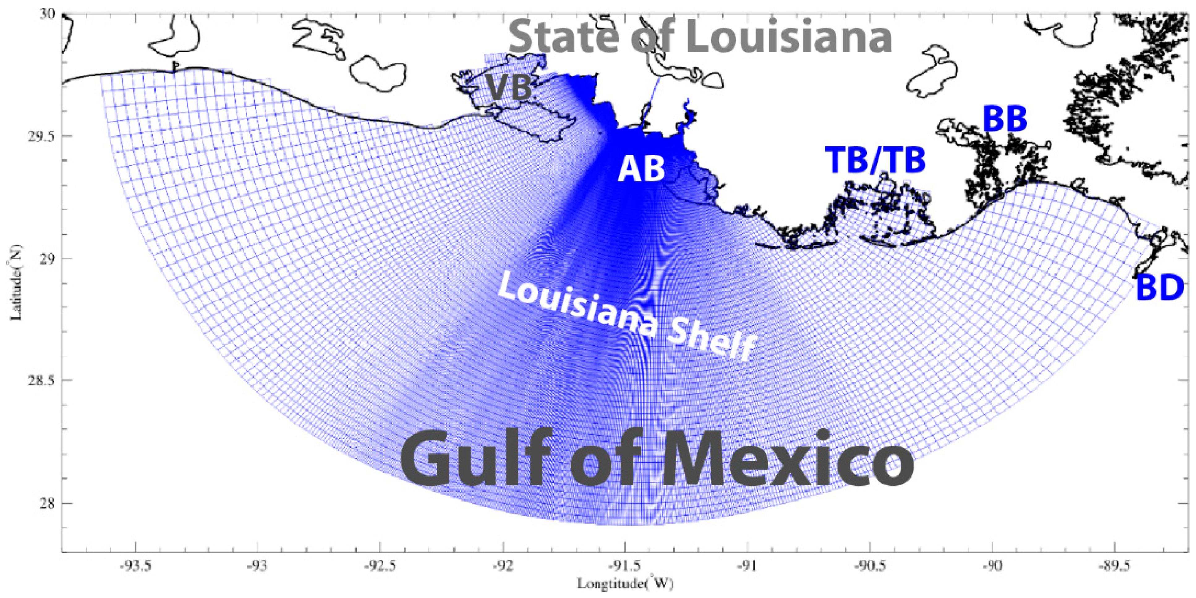
The model domain encompasses the Louisiana inner shelf from the Texas-Louisiana border to the Louisiana Bight and Mississippi River bird-foot delta (Figure 3). It covers the Atchafalaya Bay system which encompasses five contiguous bays: Vermillion Bay, West and East Cote Blanche Bays, Atchafalaya Bay, and Fourleague Bay [56,57]. The model domain is fan-shaped and centered at the WLD including the coastal, shelf, and shelf break regions. The model is divided into cells in the curvilinear horizontal orthogonal coordinate system (Figure 3; with 380 cells in the east-west and 250 cells in the north-south directions, roughly. The vertical grid is divided into 10 -layers (11 levels) with uniform thickness. The horizontal resolution ranges between 63 m and 5 km in the cross-shore direction and between 23 m and 7.75 km in the alongshore direction. Considering that the channel width ranges between 0.25 km and 2 km, there are at least 10 grids across the narrowest channel and ~90 grids across the widest channel. The resolution progressively decreases towards offshore and away from the center of the semi-circular region (Figure 3). The southern boundary is extended offshore to the shelf edge. The fan-shaped mesh allows higher-resolution cells to be placed along the inner WLD and the zones surrounding the river mouths while reducing the grid resolution offshore and near the open boundary. The water depth in this computational region ranged between 0 and 150 m. It also included land topography with a maximum height of 19.9 m above the mean sea level, allowing the model’s wet/dry capability.
The open boundary in this model is roughly an arc around the mouth of the Atchafalaya Bay (Figure 3). The model is forced by the wind on the surface and by the tide at the open boundary using nine tidal constituents from the USACE’s Eastcoast 2001 [58] computed by ADCIRC-2DDI (i.e., the depth-integrated version of the ADCIRC; [59,60,61,62,63]).
Time-dependent and spatially uniform weather data are used as forcing on the surface. These include wind and sea-level air pressure from the station FRWL1-8766072 maintained by the National Data Buoy Center (NDBC) at Fresh Water Canal Locks, LA (Figure 1). The height of the anemometer for this station is 17.4 m. Since wind speed varies with height above the water surface and considering that the standard height used in hindcasting is 10 m, we used a logarithmic velocity profile [64] to correct the wind velocity at a different height above the water ():
where z is the anemometer height in m, and is the measured wind speed in m/s. The wind velocity is then converted to wind stress as input in the model.
The model is also provided with river discharge in the lateral boundary condition. More specifically, it includes the Wax Lake Outlet (Calumet, LA; WL, USGS station #07381590) and the Lower Atchafalaya River (Morgan City, LA; LAR, USGS station #07381590). The river discharge was unidirectional since both discharge stations are located upstream away from the estuary and hence there are no flow reversals due to tidal oscillations, although surface elevation does contain tidal signals at these stations.
The initial conditions for both surface elevation and current velocity are zero. A wet/dry scheme is included using a critical depth of . To optimize the computational efficiency, the time step is set to vary automatically based on the CFL (Courant–Friedrichs–Lewy) criterion allowing the use of a larger time step during low-speed periods, but a smaller time step when the current speed is large.
3.2. Validation: Skill Assessment
The computed water level time series at 14 stations and velocity at 4 stations are compared with the observations using the correlation coefficient (CC) and skill score (SS):
in which N is the length of the time series, is the model output and is the observed value.
The skill score (SS) [65] is defined as:
Model Results with SS > 0.65 was categorized as excellent; 0.65–0.5 very good; 0.5–0.2 good; and <0.2 poor [65].
The skill assessment of the model with the combined forcing of surface wind, tide, and river discharge is calculated and summarized with the SS values shown in Table 2 and Table 3. The model performance in computing water level is in the “very good” category when compared with field observations [65,66,67,68] while the model performance to compute the current velocity at the Delta #1 and Big Hogs Bayou field sampling stations is in the “excellent” category (Table 2). The correlation coefficients are generally larger than the skill scores, consistent with [67], which showed that the skill scores are generally smaller than the square of the correlation coefficients. Since we have a relatively high skill score, our correlation coefficients are even higher, and we omit the discussion for brevity.
4. Results and Discussion
4.1. Cold Front Events
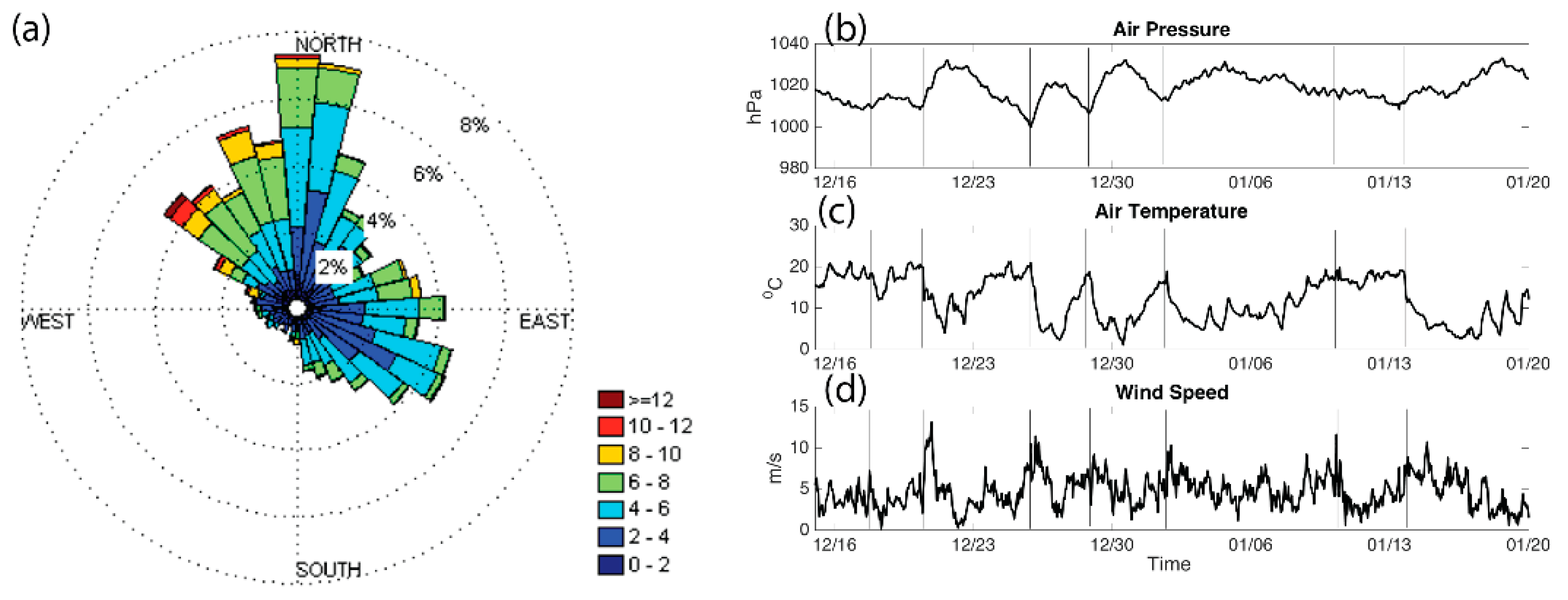
Six cold front events passed the WLD region in the study period (Table 4; Figure 4); these events, which are associated with Migrating Cyclones (MC [3,11,13]), moved southeastward across Louisiana with average speeds of ~3 m/s. Based on the distance between Terrebonne Bay and the Atchafalaya Bay (~116 km), the average time for a cold front to pass these two locations was ~11 h.
Wind direction was variable but was dominated by southeasterly (~30%), northerly (~34%), and northwesterly (~15%) winds (Figure 4). The frequency of strong winds with speeds >10.0 m/s was rare (1.2%) and mostly associated with cold front passages coming from the northwest direction. The cold front frequency was 3 to 8 days (Table 4) and was consistent with previous studies (e.g., [1,69]). Wind patterns show that each cold front event can be identified and characterized by an abrupt change in wind direction when the surface wind quickly shifts from the prefrontal southeast wind to the stronger postfrontal northwest wind. This postfrontal wind usually persists until the next cold front approaches when the wind switches to from the southern quadrants. Each cold front event recorded during the study period lasted ~2 days except the fifth event that was characterized by a prolonged north wind lasting almost 10 days after the frontal passage. The wind speed varied significantly from ~6 m/s to ~15 m/s. Before the cold front’s arrival, air pressure decreased steadily and reached the lowest value (as low as 1000 hPa) before a rapid increase up to 1040 hPa. The air pressure usually continued to increase after the front left the area (Figure 4b) as the center of another high-pressure system moved in. At the same time, the air temperature reached the lowest value after the frontal passage (Figure 4c).
4.2. Water Flow and Transport
The WLD has seven major channels or passes radiating outward (Figure 2). At the current stage of accretion, the delta is characterized by a network of secondary channels connecting primary channels to the wetlands established at high elevations along the levees and inside the lobes/islands [24]. The structure of the channel network and connection to the inundated island interiors primarily control the water circulation and flux in this distributary system [33]. Vegetation, water level, and external forcings also modulate transport patterns [36,37].
To determine the net water flux across the delta region with a network of channels, we selected a couple dozen cross-sections (Figure 2). Water transport (or volume transport at a given time) at a given section is computed by applying the following equation:
where is the horizontal velocity component perpendicular to the cross-section. The total water depth is the superposition of the local undisturbed water depth, , and surface elevation, , from the model output. L is the width of the cross-section. The accumulated total water volume over a time period is calculated by integrating Equation (12) to yield:
where is the time interval, is the initial time, and final time is . The subtidal water flux time series is obtained by applying the 6th-order Butterworth low-pass filter with a 0.6 cycle per day (CPD) cutoff frequency [70].
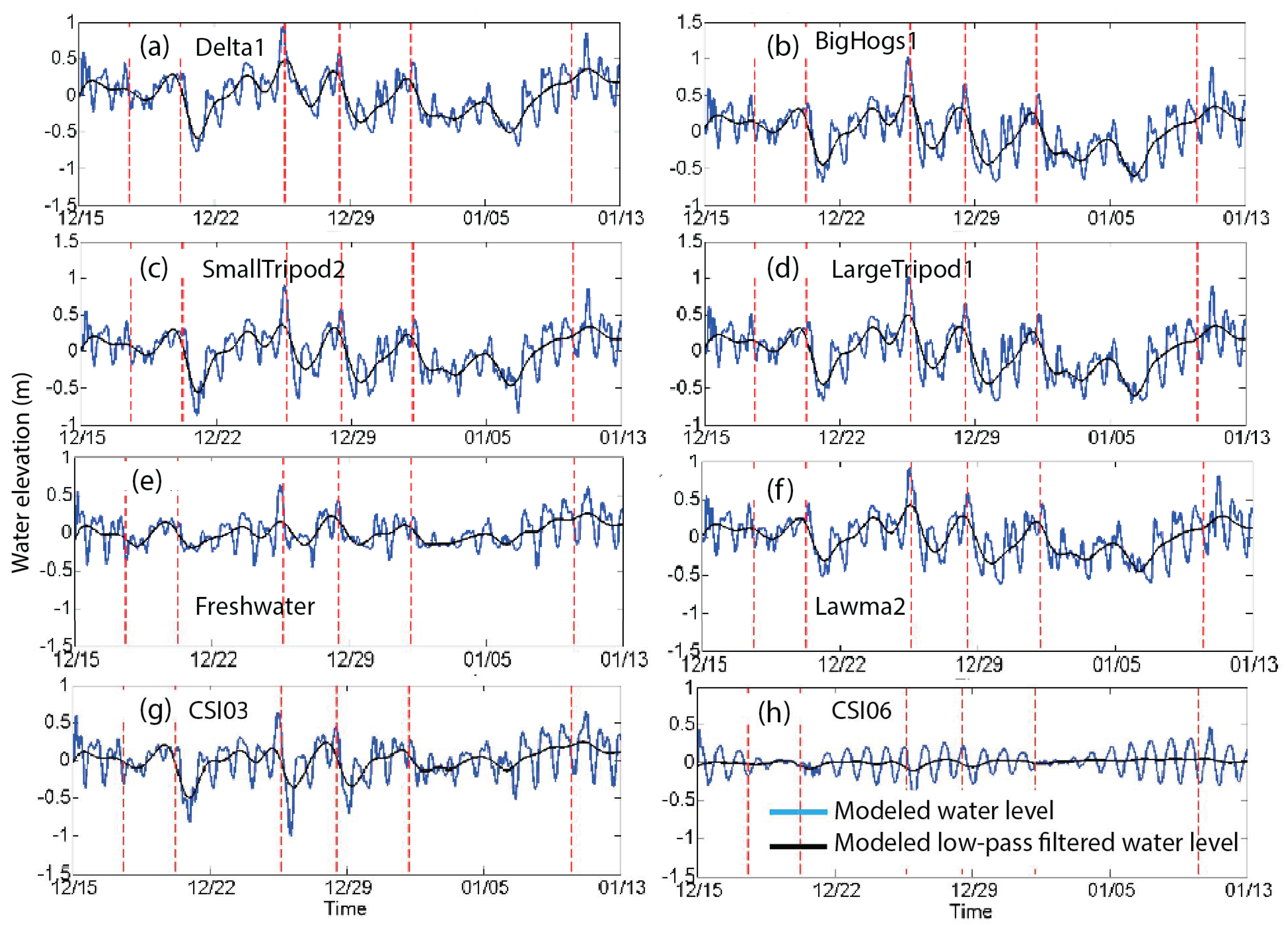
The percentage of water volume flushed out of the system during the six cold fronts ranged between 32% and 76% of the WLD’s total water volume (Table 5), this gives an average of 54.5% ± 16.8%. These values are larger than previously reported (Feng and Li, 2009), possibly because of the extremely shallow water in most of the WLD. It is interesting to note that the magnitude of water flushed out of the system is not necessarily dependent on the duration of the frontal events (41–185 h; Table 5). The maximum flushing out occurred during the third cold front event on 26 December 2012. This cold front had the lowest air pressure (Figure 4), maximum volume fluctuations, and maximum water elevation fluctuations (Figure 5).
This high percentage of water volume flushed out of the system underscores the significant impact of cold fronts in draining the system as water moves from the WLD to the Atchafalaya Bay before exiting to the adjacent continental shelf within a relatively short time [13]. This cold front-induced drainage is further facilitated by the extensive and shallow area where the average water column depth is ~2 m. The maximum percentage of water volume flushed out of the system reported by Feng and Li [13] by analyzing 29 cold front events was about 45%.
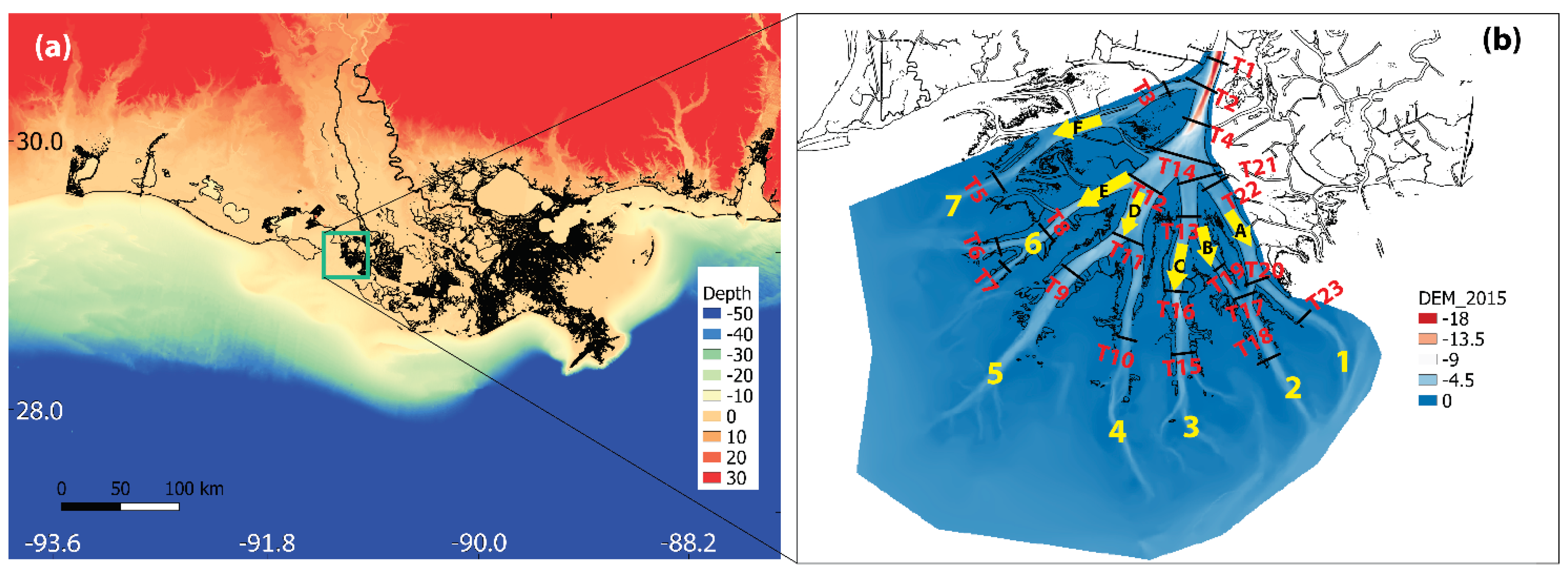
The simulated time-series water flow (and volume transport) in all seven channels show a diurnal variation and subtidal variations (e.g., Figure 5a) which are driven by the cold front wind. The cold front induced-water flow in the channels is significantly variable as the wind varies. Some general features, however, can be discerned as shown by the small portion of the total flow that is delivered to the Atchafalaya Bay via channelized discharge. For instance, of the accumulated water flux at these locations, only 50% of the volume at T14 flows into channels 4, 5, and 6 through T12. Further, 15% of the total flow is diverted into channels 2 and 3 through T15 and T18 while 10% moves to channel 1 via T23 (Figure 2). The remaining 25% is “lost” through the shallow water vegetated regions located among the main channels.
Based on the accumulated volumetric water flux results, all seven main channels contribute to water transport into the Atchafalaya Bay; although each channel (Figure 2b) contributes differently to the total flux. For example, the net transport from the Wax Lake Outlet transits through the cross-section T2 and then T3, which is the last channel located at the northwestern boundary. Once the water flow crosses into T4, it moves through the widest cross-section of that channel (~2 km) and then to T22 along channel 1. Channels 3, 4, 5, and 6 have the largest flow partition that is similar in range to previous flux estimates (e.g., [32]). The composite water flux channelized through channels 1 to 6 is the largest water flow occurring in the southern part of the delta. This area is also characterized by large extension of forested [71] and freshwater wetlands [29]. Thus, this area forms a complex spatial arrangement of wetland habitats flanked by subaqueous levees over which flow is driven by pressure gradients force [33].
The water flux balance can be expressed as:
where , , , , , , and represent the volume flux through seven main channels. The model simulations suggest that water flows into the wetland habitats account for ~25% of the total flux through the system, similar to the previous estimates by [31,72].
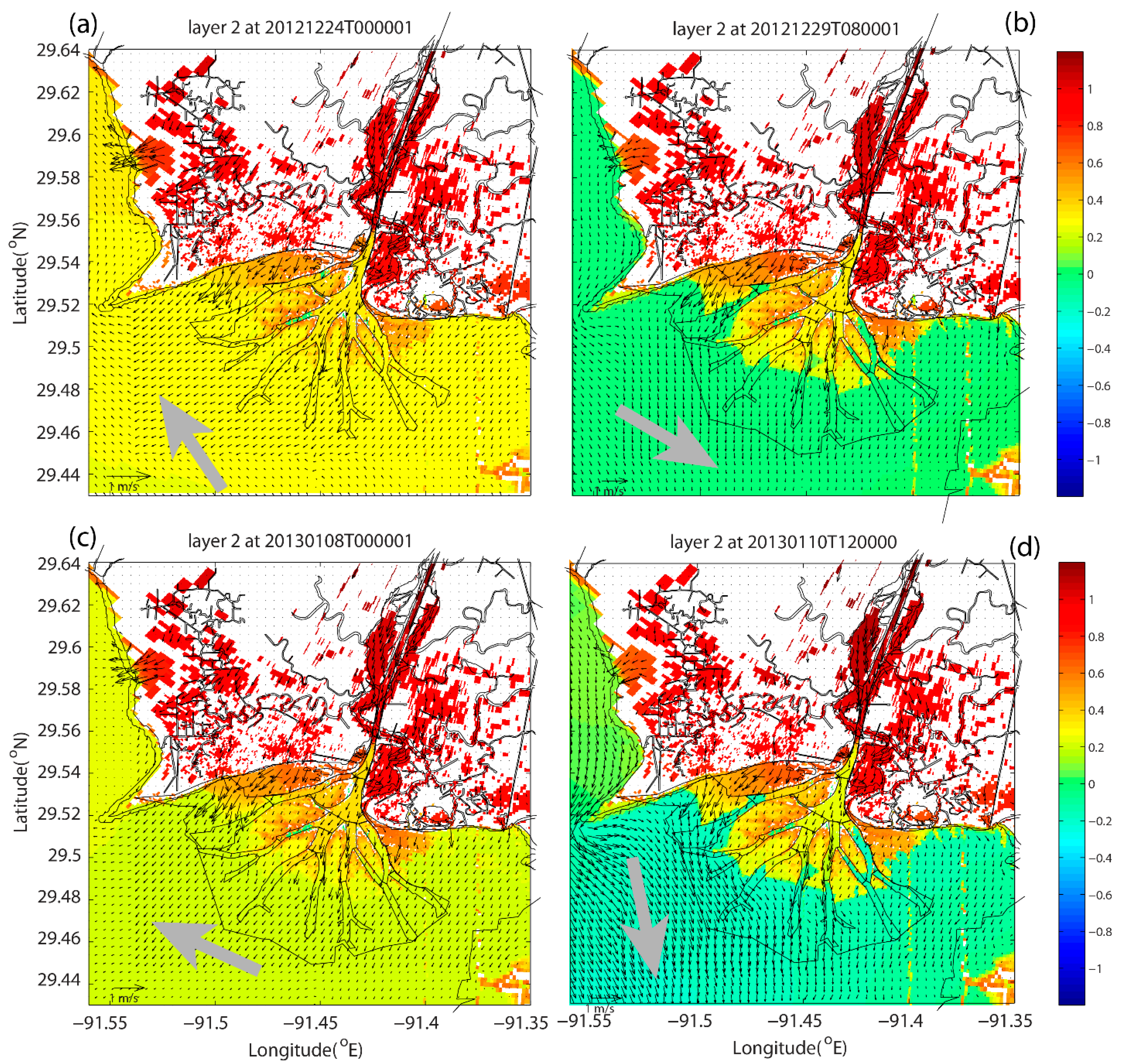
This water flow pattern can also be demonstrated by the water current maps showing both along- and cross-channel flows (Figure 6). The pre-frontal winds push the water up against the coastline, increasing the water level (Figure 6a,c); while the post-frontal winds push the water level down (Figure 6b,d). Flooding and water intrusion are evident in the very shallow or (sometimes) dry areas next to the channel bifurcations. Both wind magnitude and direction play a critical role in water transport across a wide topographic range. Our model simulations show significant water transport in the northwest to the southeast direction across the channels during strong post-frontal winds (Figure 6). As previously mentioned, the net water volume transported during these events had a major impact on vegetated and unvegetated areas inside the islands particularly with changes in the sediment deposition (Elliton et al. 2020), and thus needs to be considered when assessing ecological and biogeochemical processes in the delta lobes, e.g., denitrification [71] and wetland primary productivity [73]) in addition to predictions of the morphodynamic development that typically lack wind forcing, as suggested by [74].
4.3. Water Level Amplitude Spectrum
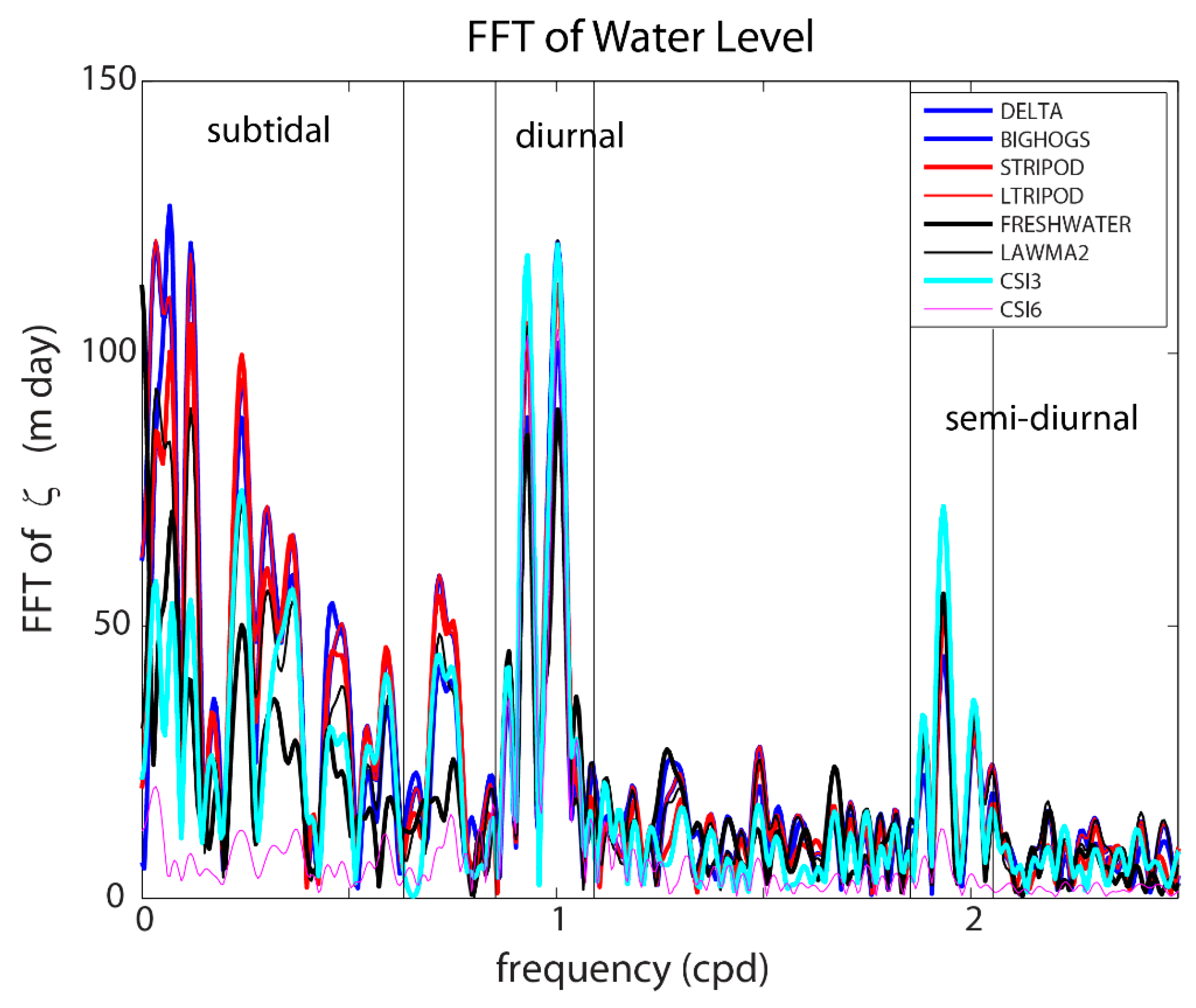
The spectrum of water levels in all field sampling stations showed a dominant diurnal tidal signal (Figure 7). Two peaks indicated the highest frequencies with values of 0.9418 CPD (or 25.48 h for one period) and 1.0009 CPD (23.79 h), close to the tidal constituents O1 (0.9295 CPD), M1 (0.9664 CPD), K1 (1.0027 CPD), S1 (1.0000 CPD), and P1 (0.9973 CPD). Although semidiurnal tidal signals were detected for most stations, their energies (see below) are lower than those observed for diurnal tides. Three major peaks were identified with frequencies of 1.884 CPD (12.74 h), 1.951 CPD (12.30 h), and 2.018 CPD (11.89 h), close to N2 (1.8960 CPD), M2 (1.9323 CPD), and S2 (2.0000 CPD). In contrast to other stations, the stations DL, BH, ST, LT, FRWL, LAW, and CSI3 (Figure 1) have relatively higher semidiurnal signals. The amplitudes of the highest semidiurnal peaks accounted for 27% to 39% of the diurnal peaks. Stations CSI3 and FRWL showed the largest semidiurnal tidal signals among all the stations. These results are consistent with other field-based water current measurements showing that areas southwest of the Atchafalaya Bay have the largest M2 tidal current across the Louisiana-Texas shelf [69]. The higher diurnal tidal components are anticipated as the region is dominated by diurnal tides [75].
The water level amplitude spectra also show periodicities longer than 2 days and are consistent with the cold front intervals. Indeed, this pattern coincides with the frequencies of cold-front-induced oscillations that are usually <0.5 CPD, and unlike tidal oscillations, cold-front-induced oscillations do not have fixed frequencies. In general, the energy is distributed throughout the low frequency range [10]. The amplitude spectra for the inshore and nearshore stations FRWL, DL, ST, LT, CSI3, BH, and LAW (Figure 1) show a strong response to wind forcing as indicated by the high-water level FFT magnitude in the 3–7 day band. In contrast, the offshore stations, e.g., CSI6, are less influenced in this range. The DL and BH spectra have similar amplitudes but slightly different patterns in the low frequency range (0–0.1 CPD) as was the case for the stations BH and LT. Further, the BH and LAW spectra have similar patterns but different amplitudes. These results indicate that although the sampling stations are in close vicinity, they are different in terms of their environment. For example, the station DL is situated in one of the main channels in the WLD and surrounded by shallow water; although BH is also in shallow waters, it is influenced by water circulation from both deltas. In contrast, the LAW station is in deeper waters close to the inner shelf (Figure 1c). There are also greater differences in velocity than in water level in response to cold front wind forcing. The greater variability in flow velocity is anticipated as the flow velocity is influenced more by the water depth.
The model results also show that the timing of the cold front is consistent with the major set-up and set-down of subtidal water level as anticipated (e.g., Atchafalaya/Vermillion Bay [13,70]; Port Fourchon [9]; and Barataria Bay [10]) (Figure 5). The variations among results from the model results (both raw results and low-pass filtered subtidal water levels) are evident in stations DL, BH, ST, LT, FRWL, LAW, CSI3, and CSI6 (Figure 5). In all cases, the pre-frontal winds from the southern quadrants caused the water level to build up. After cold fronts pass these stations, northerly winds dominate, and the water level is drawn down by the reversed wind and seaward transport of water. The variability in water level response between different events is large, ranging from <0.1 m to close to 1 m, depending on several factors: the strength and approach angle of the cold front events, wind stress, and wind direction/duration. Overall, stations DL, BH, ST, LT, FRWL, LAW, and CSI3 have relatively large variabilities compared to the other stations, apparently as a result of their relatively shallower water depths (1–5 m). The modeling results showed discernible wind-induced water level variations at all stations inside the Atchafalaya Bay where the observed water level setup was greater than 0.5 m (i.e., at DL, ST, LT, BH, FRWL, and LAW) [76] with the highest water level recorded on 26 December 2012 (Figure 5). In general, the water level variation between two successive cold front passages is caused by strong, persistent (2–3 days), and long-fetch onshore winds (>10 m/s) coming from the south and southeast quadrants. As discussed in Li et al. (2018b), the subtidal water level variation caused by cold front passages typically goes up and down over time, resembling a figure similar to a “V” or “M”.
4.4. Energy Distribution and Dominant Forcing
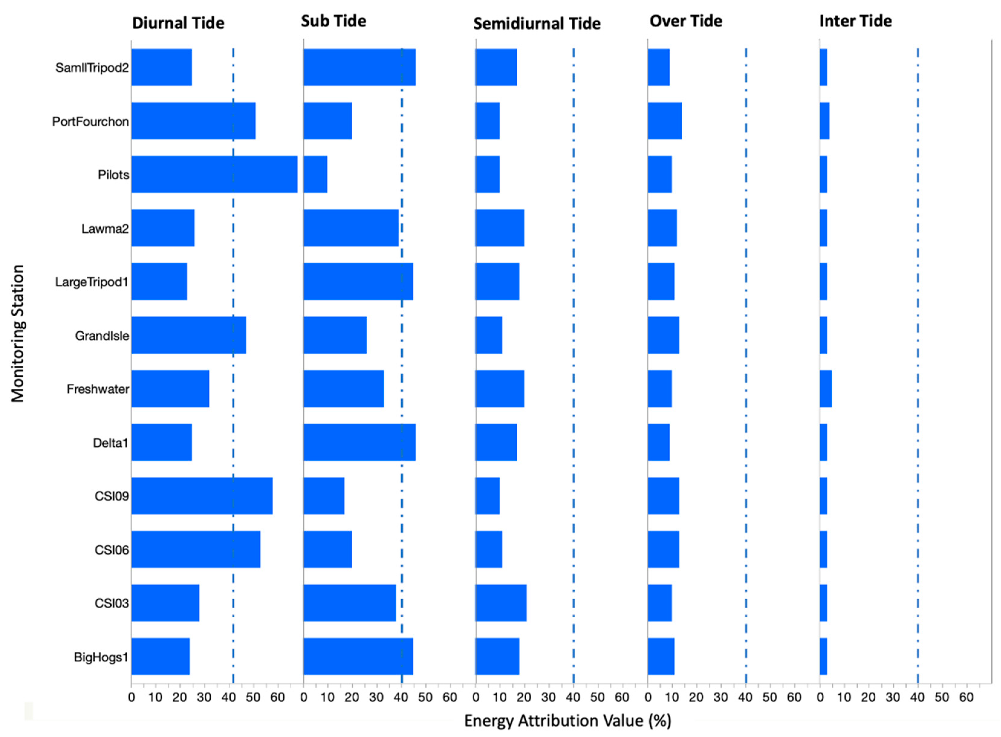
To evaluate the relative importance of various components of the hydrodynamics in the WLD region based on the numerical model results, we partitioned the energy into diurnal tidal, semi-diurnal tidal, subtidal, inter-tidal, and over-tidal components [10]. This is done based on the power spectrum of the water level or water velocity. The partitioning is possible because each of the five components has spectrum regimes that are mostly non-overlapping, given that our interest in the cold front effect is limited to the subtidal variations (not a short time scale variation due to, e.g., a wind gust over a few minutes or a few hours).
The results show that generally speaking, the energy partitioning varies among stations (Figure 8) but with some general patterns: the diurnal energy is generally comparable to the subtidal energy outside of the WLD region. This however is complicated by the variabilities of all components. For example, the diurnal tidal energy contribution ranges from 24–68% of the total energy while the subtidal and semidiurnal ranges from 10–46% and 10% and 21%, respectively. The diurnal tide is dominant in six out of the twelve stations followed by the subtidal component (mainly due to wind and nonlinearity). Those stations are located east of the Atchafalaya-Wax Lake complex. In contrast, the stations CSI3 and FRWL located in the western region have similar values among diurnal, semidiurnal tide, and subtidal components. What is more striking is that the energy allocation in stations within the WLD shows that the subtidal component accounted for 46–66% of total energy, which is larger than the diurnal tidal contribution of only 13–25% of the total energy. This energy partition confirms that seasonal pulsing in weather patterns—caused by the impact of atmospheric cold front passages across the Wax Lake deltaic region—is critical in regulating water circulation and the total net water flux at local scales between the delta and the Atchafalaya/Inner coastal shelf complex [10].
5. Conclusions
Results from the 3-D ECOM-si model show that both tidal and subtidal variations of water level and current velocity in the WLD and adjacent deeper open water areas are consistent with observations during a period with six cold fronts occurring between 15 December 2012 and 20 January 2013. The water transport through the delta distributary channel network under cold front weather is not solely confined within the channels; water can also have a significant lateral exchange thus hydrologically connecting the channels through the extensive wetland habitats inside the delta lobes/islands. This inter-channel lateral flow can account for approximately 25% of the total flow through the main WLD channels. During these events, the subtidal water level increased during the prefrontal period caused by the onshore southerly wind, reaching a maximum value (~1 m), and then started to drop 6–9 h prior to the frontal passage. Similarly, the subtidal influx velocity reached the highest value (~0.6 m/s) before the outward flow was developed by wind forcing from different directions after the frontal passage. The subtidal outflow reached its maximum five to eleven hours after the frontal passage because of the persistent and relatively strong winds (which can exceed 10 m/s) from the northern quadrants; the outflow, however, started to decrease as the wind weakened. The northerly winds promoted significant water flushing out of the bays as previously reported [13,70]. These cold-front-induced flushing events can last from ~40 to185 h in the WLD. Indeed, 32 to 76% of the total water in the WLD was flushed out during these cold front events analyzed in our study. This is a larger range than previously reported [13].
Finally, a spectral energy analysis revealed that both tidal and subtidal energies vary substantially. The tidal energy ranges between 20% and 70% of the total energy, while the subtidal energy varies between 10% and 45% of the total energy (Figure 8). What is most important is that within the WLD region, the weather-induced subtidal energy (46–66% of the total) is much greater than the diurnal tidal energy (13–25% of the total). This is apparently due to the shallow water in the WDL region. The shallow water (~1–2 m) implies a high nonlinear parameter (water level change divided by mean water depth) and thus a nonlinear process. The wind associated with cold fronts in winter is the main factor controlling water circulation in the WLD and is a major driver in the spatial configuration of the channel network and delta progradation rates. During the study period, river discharge had little impact on the water level and water exchange when compared to the tidal and wind effects. These results indicate that water circulation within the WLD shallow system (<2 m) is primarily dominated by wind, especially during cold fronts. Although hurricanes can cause more significant acute impacts, cold fronts are more frequent, and their integrated effect cannot be ignored when assessing hydrodynamic patterns at the regional scale; especially since cold fronts have a significant effect on shaping the WLD morphology. As discussed in [2], there were more than 1600 cold frontal events influencing the study area over a period of 40 years. The subtidal energy is more important in the WLD than in the offshore areas, thus underlying the functional role of cold fronts in this coastal region since they become more important than tides in flushing this young delta as it continues to develop and expand—even as sea level rise continues to increase in the NGOM [77,78].
Author Contributions
Conceptualization, C.L.; methodology, Q.Z., J.L. and C.L.; software, Q.Z., J.L. and C.L.; validation, Q.Z. and W.H.; formal analysis, Q.Z.; investigation, Q.Z.; resources, C.L.; data curation, Q.Z.; writing—original draft preparation, Q.Z.; writing—review and editing, C.L., W.H., M.H. and V.H.R.-M.; visualization, Q.Z. and M.H.; supervision, C.L.; project administration, C.L.; funding acquisition, C.L., M.H. and V.H.R.-M. All authors have read and agreed to the published version of the manuscript.
Funding
This research was funded by NOAA (NA16NOS0120018; NOS-IOOS-2016-2004378) to C.L., by the National Science Foundation Grant EAR-2023443 awarded to M.H. and C.L. It was also supported by National Science Foundation (NSF OCE-1140307; NSF-NERC 1736713 and 1737274) and the State of Louisiana Coastal Protection and Restoration Authority through the CPRA Interagency Agreement No. 2503-11-08, CFMS Contract No. 695678 with Louisiana State University awarded to C.L., V.R.H.-M. participation in the preparation of this publication was supported by the US Department of the Interior, South Central-Climate Adaptation Center (Cooperative Agreement #G12AC00002) The statements, findings, and conclusions are those of the authors and do not necessarily reflect the views of the funding agencies.
Institutional Review Board Statement
Not applicable.
Informed Consent Statement
Not applicable.
Data Availability Statement
The weather data used in this work can be found in the links of the agency’s websites as indicated in the description. The data generated in this work can be found at https://oceandynamics.lsu.edu/data/WaxLakeDelta.htm (accessed on 7 March 2022).
Acknowledgments
The authors thank Changsheng Chen for his generosity in allowing us to use his modified ECOM-si model. We thank Harry Roberts for discussions and to Eddie Weeks for field work. The authors acknowledge the Coastal Studies Institute Field Support Group personnel for fabricating, deploying, and retrieving the instrumented tripod used in this investigation.
Conflicts of Interest
The authors declare no conflict of interest.
References
- Fernandez-Partagas, J.; Mooers, C.N.K. A synoptic study of winter cold fronts in Florida. Mon. Weather. Rev. 1975, 103, 742–744. [Google Scholar] [CrossRef] [Green Version]
- Li, C.; Huang, W.; Wu, R.; Sheremet, A. Weather induced quasi-periodic motions in estuaries and bays: Meteorological tide. China Ocean. Eng. 2020, 34, 299–313. [Google Scholar] [CrossRef]
- Roberts, H.H.; Huh, O.K.; Hsu, S.A.; Rouse, L.J.; Rickman, D.A. Impact of cold-front passages on geomorphic evolution and sediment dynamics of the complex Louisiana coast. In Coastal Sediments ’87, Proceedings of the Specialty Conference on Advances in Understanding of Coastal Sediment Processes, New Orleans, LA, USA, 12–14 May 1987; American Society of Civil Engineers: Reston, VA, USA, 1987; pp. 1950–1963. [Google Scholar]
- Mossa, J.; Roberts, H.H. Synergism of riverine and winter storm-related sediment transport processes in Louisiana’s coastal wetlands. Trans. Gulf Coast Assoc. Geol. Soc. 1990, 40, 635–642. [Google Scholar]
- Lin, J.; Li, C.; Boswell, K.M.; Kimball, M.; Rozas, L. Examination of Winter Circulation in a Northern Gulf of Mexico Estuary. Estuaries Coasts 2016, 39, 1–21. [Google Scholar] [CrossRef]
- Huang, W.; Li, C. Cold front driven flows through multiple inlets of Lake Pontchartrain Estuary. J. Geophys. Res. 2017. [Google Scholar] [CrossRef] [Green Version]
- Huang, W.; Li, C. Spatial variation of cold front wind-driven circulation and quasi-steady state balance in Lake Pontchartrain Estuary. Estuar. Coast. Shelf Sci. 2019, 224, 154–170. [Google Scholar] [CrossRef]
- Li, C.; Huang, W.; Chen, C.; Lin, H. Flow regimes and adjustment to wind-driven motions in Lake Pontchartrain: A modeling experiment using FVCOM. J. Geophys. Res.—Ocean 2018. [Google Scholar] [CrossRef]
- Li, C.; Weeks, E.; Huang, W.; Milan, B.; Wu, R. Weather-Induced Transport through a Tidal Channel Calibrated by an Unmanned Boa. J. Atmos. Ocean. Technol. 2018, 35, 261–279. [Google Scholar] [CrossRef]
- Li, C.; Huang, W.; Milan, B. Atmospheric cold front induced exchange flows through a microtidal multi-inlet bay: Analysis using multiple horizontal ADCPs and FVCOM simulations. J. Atmos. Ocean. Technol. 2019, 36, 443–472. [Google Scholar] [CrossRef]
- Roberts, H.H.; Huh, O.K.; Hsu, S.A.; Rouse, L.J., Jr.; Rickman, D.A. Winter storm impact on the Chenier Plain Coast of Southwestern Louisiana. Gulf Coast Assoc. Geol. Soc. Trans. 1989, 39, 515–522. [Google Scholar]
- Pepper, D.A.; Stone, G.W. Hydrodynamics and sedimentary responses to two contrasting winter storms on the inner shelf of the northern Gulf of Mexico. Mar. Geol. 2004, 210, 43–62. [Google Scholar] [CrossRef]
- Feng, Z.; Li, C. Cold-front-induced flushing of the Louisiana Bays. J. Mar. Syst. 2010, 82, 252–264. [Google Scholar] [CrossRef]
- Wellner, R.; Beaubouef, R.; van Wagoner, J.; Roberts, H.H.; Sun, T. Jet-plume depositional bodies: The primary building blocks of Wax Lake Delta. Trans. Gulf Coast Assoc. Geol. Soc. 2005, 55, 867–909. [Google Scholar]
- Falcini, F.; Jerolmack, D.J. A potential vorticity theory for the formation of elongate channels in river deltas and lakes. J. Geophys. Res. 2010, 115, F04038. [Google Scholar] [CrossRef] [Green Version]
- Edmonds, D.A.; Paola, C.; Hoyal, D.C.J.D.; Sheets, B.A. Quantitative metrics that describe river deltas and their channel networks. J. Geophys. Res. 2011, 116, F04022. [Google Scholar] [CrossRef]
- Schlemon, R.J. Subaqueous delta formation-Atchafalaya Bay, Louisiana. In Deltas: Models for Exploration; Broussard, M.L., Ed.; Houston Geological Society: Houston, TX, USA, 1975; pp. 209–221. [Google Scholar]
- Roberts, H.H.; Walker, N.; Cunningham, R.; Kemp, G.P.; Majersky, S. Evolution of sedimentary architecture and surface morphology: Atchafalaya and Wax Lake deltas, Louisiana. Trans. Gulf Coast Assoc. Geol. Soc. 1997, 47, 477–484. [Google Scholar]
- Roberts, H.H.; Coleman, J.M.; Bentley, S.J.; Walker, N. An embryonic major delta lobe: A new generation of delta studies in the Atchafalaya-Wax Lake delta systems. GCAGS/GCSSEPM Trans. 2003, 53, 690–703. [Google Scholar]
- Edmonds, D.; Slingerland, R. Mechanics of river mouth bar formation: Implications for the morphodynamics of delta distributary networks. J. Geophys. Res. 2007, 112, F02034. [Google Scholar] [CrossRef] [Green Version]
- Meselhe, E.; Sadid, K.; Khadka, A. Sediment Distribution, Retention and Morphodynamic Analysis of a River-Dominated Deltaic System. Water 2021, 13, 1341. [Google Scholar] [CrossRef]
- Rivera-Monroy, V.H.; Elliton, C.; Narra, S.; Meselhe, E.; Zhao, X.; White, E.; Sasser, C.E.; Visser, J.M.; Meng, X.; Wang, H.; et al. Wetland Biomass and Productivity in Coastal Louisiana: Base Line Data (1976–2015) and Knowledge Gaps for the Development of Spatially Rehabilitation Initiatives. Water 2019, 11, 2054. [Google Scholar] [CrossRef] [Green Version]
- Vargas-Lopez, I.A.; Rivera-Monroy, V.H.; Day, J.W.; Whitbeck, J.; Maiti, K.; Madden, C.J.; Trasviña-Castro, A. Assessing Chlorophyll a Spatiotemporal Patterns Combining In Situ Continuous Fluorometry Measurements and Landsat 8/OLI Data Across the Barataria Basin (Louisiana, USA). Water 2021, 13, 512. [Google Scholar] [CrossRef]
- Elliton, C.; Xu, K.; Rivera-Monroy, V.H. The Impact of Biophysical Processes on Sediment Transport in the Wax Lake Delta (Louisiana, USA). Water 2020, 12, 2072. [Google Scholar] [CrossRef]
- Roberts, H.H.; Beaubouef, R.T.; Walker, N.D.; Stone, G.W.; Bentley, S.; Shermet, A.; van Heerden, I.I. San-rich bayhead deltas in Atchafalaya Bay (Louisiana): Winnowing by cold front forcing. In Proceedings of the Coastal Sediments’ 03, Clearwater, FL, USA, 18–23 May 2003; pp. 1–15. [Google Scholar]
- Shaw, J.B.; Mohrig, D.; Whitman, S.K. The Morphology and Evolution of Channels on the Wax Lake Delta. J. Geophys. Res. 2013, 118, 1–22. [Google Scholar] [CrossRef]
- Shaw, J.B.; Mohrig, D.; Wagner, R.W. Flow patterns and morphology of a prograding river delta. J. Geophys. Res. Earth Surf. 2016, 2015JF003570. [Google Scholar] [CrossRef]
- Kim, W.; Mohrig, D.; Twilley, R.; Paola, C.; Parker, G. Is it feasible to build new land in the Mississippi River delta? EOS Trans. Am. Geophys. Union 2009, 90, 373–374. [Google Scholar] [CrossRef]
- Carle, M.V.; Sasser, C.E. Productivity and resilience: Long-term trends and storm-driven fluctuations in the plant community of the accreting Wax Lake Delta. Estuaries Coasts 2016, 39, 406–422. [Google Scholar] [CrossRef]
- Li, C.; Weeks, E.; Rego, J.L. In situ measurements of saltwater flux through tidal passes of Lake Pontchartrain estuary by Hurricanes Gustav and Ike in September 2008. Geophys. Res. Lett. 2009, 36, L19609. [Google Scholar] [CrossRef]
- Hiatt, M.; Passalacqua, P. Hydrological connectivity in river deltas: The first-order importance of channel-island exchange. Water Resour. Res. 2015, 51, 2264–2282. [Google Scholar] [CrossRef] [Green Version]
- Hiatt, M.; Castañeda-Moya, E.; Twilley, R.; Hodges, B.R.; Passalacqua, P. Channel-island connectivity affects exposure time distributions in a coastal river delta. Water Resour. Res. 2018, 54. [Google Scholar] [CrossRef]
- Hiatt, M.; Passalacqua, P. What controls the transition from confined to unconfined flow? Analysis of hydraulics in a coastal river delta. J. Hydraul. Eng. 2017, 143. [Google Scholar] [CrossRef]
- Hiatt, M. A Network-Based Analysis of River Delta Surface Hydrology: An Example from Wax Lake Delta. Master’s Dissertation, University of Texas at Austin, Austin, TX, USA, 2013. [Google Scholar]
- Musner, T.; Bottacin-Busolin, A.; Zaramella, M.; Marion, A. A contaminant transport model for wetlands accounting for distinct residence time bimodality. J. Hydrol. 2014, 515, 237–246. [Google Scholar] [CrossRef]
- Christensen, A.; Twilley, R.R.; Willson, C.S.; Castañeda-Moya, E. Simulating hydrological connectivity and water age within a coastal deltaic floodplain of the Mississippi River Delta. Estuar. Coast. Shelf Sci. 2020, 245, 106995. [Google Scholar] [CrossRef]
- Sendrowski, A.; Castañeda-Moya, E.; Twilley, R.; Passalacqua, P. Biogeochemical and Hydrological Variables Synergistically Influence Nitrate Variability in Coastal Deltaic Wetlands. J. Geophys. Res. Biogeosci. 2021, 126, e2020JG005737. [Google Scholar] [CrossRef]
- Li, Y.; Li, C.; Li, X. Remote Sensing Studies of Suspended Sediment Concentration Variations in a Coastal Bay During the Passages of Atmospheric Cold Fronts. IEEE J. Sel. Top. Appl. Earth Obs. Remote Sens. 2017, 10, 2608–2622. [Google Scholar] [CrossRef]
- Hiatt, M.; Snedden, G.; Day, J.W.; Rohli, R.; Nyman, J.A.; Lane, R.; Sharp, L.A. Drivers and impacts of water level fluctuations in the Mississippi River delta: Implications for delta restoration. Estuar. Coast. Shelf Sci. 2019. [Google Scholar] [CrossRef]
- Knights, D.; Sawyer, A.H.; Barnes, R.T.; Piliouras, A.; Schwenk, J.; Edmonds, D.A.; Brown, A.M. Nitrate Removal Across Ecogeomorphic Zones in Wax Lake Delta, Louisiana (USA). Water Resour. Res. 2020, 56, e2019WR026867. [Google Scholar] [CrossRef]
- Walker, N.D.; Hammack, A.B. Impacts of winter storms on circulation and sediment transport: Atchafalaya-Vermilion Bay Region, Louisiana. J. Coast. Res. 2000, 16, 996–1010. [Google Scholar]
- Walker, N.D. Wind and Eddy Related Circulation on the Louisiana/Texas Shelf and Slope Determined from Satellite and In-Situ Measurements: October 1993–August 1994; College of the Coast & Environment: Baton Rouge, LA, USA, 2002. [Google Scholar]
- Roberts, H.H.; Walker, N.; Sheremet, A.; Stone, G.W. Effects of Cold Fronts on Bayhead Delta Development: Atchafalaya Bay, Louisiana, USA, High Resolution Morphodynamics and Sedimentary Evolution of Estuaries, Coastal Systems and Continental Margins; Springer: Dordrecht, The Netherlands, 2005; Volume 8, pp. 269–298. [Google Scholar]
- Blumberg, A.F. A Primer for ECOM-si; Technical Report; HydroQual, Inc.: Mahwah, NJ, USA, 1994; p. 66. [Google Scholar]
- Zhang, Q. Numerical Simulation of Cold Front Related Hydrodynamics of Wax Lake Delta. Ph.D. Dissertation, Louisiana State University, Baton Rouge, LA, USA, 2015; p. 210. [Google Scholar]
- Chen, C.; Zhu, J.; Ralph, E.; Green, S.A.; Budd, J.W.; Zhang, F.Y. Prognostic modeling studies of the Keweenaw Current in Lake Superior, part I: Formation and evolution. J. Phys. Oceanogr. 2001, 31, 379–395. [Google Scholar] [CrossRef]
- Chen, C.; Zhu, J.; Zheng, L.; Ralph, E.; Budd, J.W. A Non-orthogonal Primitive Equation Coastal Ocean Circulation Model: Application to Lake Superior. J. Great Lakes Res. 2004, 30 (Suppl. 1), 41–54. [Google Scholar] [CrossRef]
- Blumberg, A.F.; Mellor, G.L. A Description of a Three-Dimensional Coastal Ocean Circulation Model. In Three-Dimensional Coastal Ocean Models; Heaps, N.S., Ed.; American Geophysical Union: Washington, DC, USA, 1987; Volume 4, pp. 1–16. [Google Scholar]
- Zheng, L.; Chenb, C.; Zhang, F.Y. Development of water quality model in the Satilla River Estuary, Georgia. Ecol. Model. 2004, 178, 457–482. [Google Scholar] [CrossRef]
- Chen, C.; Huang, H.; Beardsley, R.C.; Liu, H.; Xu, Q.; Cowles, G. A finite volume numerical approach for coastal ocean circulation studies: Comparisons with finite difference models. J. Geophys. Res. 2007, 112, C03018. [Google Scholar] [CrossRef]
- Lyu, H.; Zhu, J. Impact of the bottom drag coefficient on saltwater intrusion in the extremely shallow estuary. J. Hydrol. 2018, 557, 838–850. [Google Scholar] [CrossRef]
- Tian, R.; Chen, C. Influence of model geometrical fitting and turbulence parameterization on phytoplankton simulation in the Gulf of Maine. Deep-Sea Res. II 2006, 53, 2808–2832. [Google Scholar] [CrossRef]
- Mellor, G.L.; Yamada, T. Development of a turbulence closure model for geophysical fluid problem. Rev. Geophys. 1982, 20, 851–875. [Google Scholar] [CrossRef] [Green Version]
- Galperin, B.; Kantha, L.H.; Hassid, S.; Rosati, A. A quasi-equilibrium turbulent energy model for geophysical flows. J. Atmos. Sci. 1988, 45, 55–62. [Google Scholar] [CrossRef] [Green Version]
- Smagorinsky, J. General circulation experiments with the primitive equations. Mon. Weather. Rev. 1963, 91, 99–164. [Google Scholar] [CrossRef]
- Cobb, M.; Keen, T.R.; Walker, N.D. Modeling the circulation of the Atchafalaya Bay system during winter cold front events. Part 1: Model description and validation. J. Coast. Res. 2008, 24, 1036–1047. [Google Scholar] [CrossRef]
- Cobb, M.; Keen, T.R.; Walker, N.D. Modeling the circulation of the Atchafalaya Bay system, part 2: River plume dynamics during cold fronts. J. Coast. Res. 2008, 24, 1048–1062. [Google Scholar] [CrossRef]
- Mukai, A.Y.; Westerink, J.J.; Luettich, R.A. Guidelines for Using Eastcoast 2001 Database of Tidal Constituents within Western North Atlantic Ocean, Gulf of Mexico and Caribbean, Coastal and Hydraulics Engineering; Technical Note CHETN-IV-40; U.S. Army Engineer Research and Development Center: Vicksburg, MS, USA, 2001. [Google Scholar]
- Westerink, J.J. Tidal Prediction in the Gulf of Mexico/Galveston Bay Using Model ADCIRC-2DDI; Contractors Report; US Army Engineer Waterways Experiment Station: Vicksburg, MS, USA, 1993. [Google Scholar]
- Westerink, J.J.; Blain, C.A.; Luettich, R.A., Jr.; Scheffner, N.W. ADCIRC: An Advanced Three-Dimensional Circulation Model for Shelves Coasts and Estuaries, Report 2: Users Manual for ADCIRC-2DDI; Dredging Research Program Technical Report DRP-92-6; U.S. Army Engineers Waterways Experiment Station: Vicksburg, MS, USA, 1994; 156p. [Google Scholar]
- Westerink, J.J.; Luettich, R.A., Jr.; Scheffner, N.W. ADCIRC: An Advanced Three-Dimensional Circulation Model for Shelves Coasts and Estuaries, Report 3: Development of a Tidal Constituent Data Base for the Western North Atlantic and Gulf of Mexico, Dredging Research Program; Technical Report DRP-92-6; U.S. Army Engineers Waterways Experiment Station: Vicksburg, MS, USA, 1993; 154p. [Google Scholar]
- Mukai, A.Y.; Westerink, J.J.; Luettich, R.A., Jr. Guidelines for Using the Eastcoast, 2001, Database of Tidal Constituents within the Western North Atlantic Ocean, Gulf of Mexico and Caribbean Sea; Technical Note (IV–XX); U.S. Army Engineer Research and Development Center, Coastal and Hydraulics Laboratory: Vicksburg, MS, USA, 2002; 24p. [Google Scholar]
- Mukai, A.Y.; Westerink, J.J.; Luettich, R.A., Jr.; Mark, D. Eastcoast, 2001, a Tidal Constituent Database for the Western North Atlantic, Gulf of Mexico and Caribbean Sea; Technical Report, ERDC/CHL TR-02-24; U.S. Army Engineer Research and Development Center, Coastal and Hydraulics Laboratory: Vicksburg, MS, USA, 2002; 201p. [Google Scholar]
- Kamphuis, J.W. Introduction to Coastal Engineering and Management; World Scientific: Singapore, 2000. [Google Scholar]
- Allen, J.I.; Somerfield, P.J.; Gilbert, F.J. Quantifying uncertainty in high-resolution coupled hydrodynamic-ecosystem models. J. Mar. Syst. 2007, 64, 3–14. [Google Scholar] [CrossRef]
- Liu, Y.; MacCready, P.; Hickey, B.M.; Dever, E.P.; Kosro, P.M.; Banas, N.S. Evaluation of a coastal ocean circulation model for the Columbia River plume in summer 2004. J. Geophys. Res. 2009, 114, C00B04. [Google Scholar] [CrossRef] [Green Version]
- Murphy, A.H. Skill scores based on the mean square error and their relationships to the correlation coefficient. Mon. Weather. Rev. 1988, 116, 2417–2424. [Google Scholar] [CrossRef]
- Ralston, D.K.; Geyer, W.R.; Lerczak, J.A. Structure, variability, and salt flux in a strongly forced salt wedge estuary. J. Geophys. Res. 2010, 115, C06005. [Google Scholar] [CrossRef] [Green Version]
- DiMarco, S.F.; Reid, R.O. Characterization of the principal tidal current constituents on the Texas-Louisiana shelf. J. Geophys. Res. 1998, C103, 3093–3109. [Google Scholar] [CrossRef]
- Li, C.; Roberts, H.H.; Stone, G.W. Wind surge and saltwater intrusion and Atchafalaya Bay during onshore winds prior to cold front passage. Hydrobiologia 2011, 658, 27–39. [Google Scholar] [CrossRef]
- Upreti, L.; Rivera-Monroy, V.H.; Maiti, K.; Giblin, A.; Geaghan, J.P. Emerging wetlands from river diversions can sustain high denitrification rates in a coastal delta. J. Geophys. Res. Biogeosci. 2021, 126, e2020JG006217. [Google Scholar] [CrossRef]
- Buttles, J.; Mohrig, D.; Nittrouer, J.; McElroy, B.; Baitis, E.; Allison, M.; Paola, C.; Parker, G.; Kim, W. Partitioning of water discharge by distributary channels in the prograding, Wax Lake Delta, coastal Louisiana, USA. In AGU Fall Meeting Abstracts; American Geophysical Union: Washington, DC, USA, 2007. [Google Scholar]
- Carle, M. Spatial Structure and Dynamics of the Plant Communities in a Pro-Grading River Delta: Wax Lake Delta, Atchafalaya Bay, Louisiana. Ph.D. Thesis, Louisiana State University, Baton Rouge, LA, USA, 2013; 73p. Available online: https://digitalcommons.lsu.edu/gradschool_dissertations/73 (accessed on 7 March 2022).
- Geleynse, N.; Hiatt, M.; Sangireddy, H.; Passalacqua, P. Identifyingenvironmental controls on the shore-line of a natural river delta. J. Geo-Phys. Res. Earth Surf. 2015, 120, 877–893. [Google Scholar] [CrossRef]
- Kantha, L. Barotropic tides in the Gulf of Mexico. Circulation in the Gulf of Mexico: Observations and Models. Geophys. Monogr. Amer. Geophys. Union 2005, 161, 159–163. [Google Scholar] [CrossRef]
- Van Heerden, I.L.I. Deltaic Sedimentation in Eastern Atchafalaya Bay, Louisiana. Ph.D. Dissertation, Department of Marine Sciences, Louisiana State University, Baton Rouge, LA, USA, 1983; p. 151. [Google Scholar]
- Kolker, A.S.; Allison, M.A.; Hameed, S. An evaluation of subsidence rates and sea-level variability in the northern Gulf of Mexico. Geophys. Res. Lett. 2011, 38. [Google Scholar] [CrossRef]
- Törnqvist, T.E.; Jankowski, K.L.; Li, Y.-X.; González, J.L. Tipping points of Mississippi Delta marshes due to accelerated sea-level rise. Sci. Adv. 2020, 6, eaaz5512. [Google Scholar] [CrossRef]
Figure 1.
Map of the study region and field sites. (a) The Louisiana coast and observational stations in the northern GOM. NOAA, WAVCIS, field ADCP, and USGS stations. BH: Big Hog Bayou; DL: Delta #1; LAW: LAWMA; BE: Berwick; FRWL: Freshwater Canal Locks; GI: Grand Isle; PS: Pilot’s Station East, SW Pass; PI: Pilottown; PF: Port Fourchon; ST: Small Tripod; LT: large tripod; WL: Wax Lake Outlet at Calumet; and LAR: Lower Atchafalaya River at Morgan City. (b) Inset showing the study region. (c) Zoomed-in view of the box in (a) detailing the stations in the Wax Lake region. The latitude and longitude for each station are listed in Table 1.

Figure 2.
Bathymetry used in the model. (a) Depths are given with respect to the reference level (MSL in this study) and negative values are below reference level (MSL). The coordinates are longitude and latitude. The green box indicates the location of the WLD. (b) Zoomed in view of the green box of (a). The yellow numbers 1 to 7 are used to indicate the seven channels from east to west. The red labels, T1 to T23, indicate cross-sectional transect locations along the delta channels used for model result analysis.

Figure 3.
The 380 × 250 curvilinear model grid of the Atchafalaya-WLD system. VB: Vermilion Bay; AB: Atchafalaya Bay; TB/TB: Timbalier Bay/Terrebonne Bay; BB: Barataria Bay; BD: Birdfoot Delta.
Figure 3.
The 380 × 250 curvilinear model grid of the Atchafalaya-WLD system. VB: Vermilion Bay; AB: Atchafalaya Bay; TB/TB: Timbalier Bay/Terrebonne Bay; BB: Barataria Bay; BD: Birdfoot Delta.

Figure 4.
(a) Wind rose, (b) sea-level air pressure, (c) temperature, and (d) wind speed from FRWL between 15 December 2012 and 20 January 2013. Vertical lines indicate the timing of cold front passages (b–d). Note that the lowest air pressure occurred right at the third frontal passage.
Figure 4.
(a) Wind rose, (b) sea-level air pressure, (c) temperature, and (d) wind speed from FRWL between 15 December 2012 and 20 January 2013. Vertical lines indicate the timing of cold front passages (b–d). Note that the lowest air pressure occurred right at the third frontal passage.

Figure 5.
Modeled water levels at eight stations. Subplots (a–h) are water level at Delta 1, BigHogs1, SmallTripod2, LargeTripod1, Freshwater, Lawma2, CSI03, and CSI06, respectively. The low-pass filtered results are also shown. The red dashed lines indicate the timing of the frontal passage. Note that the maximum water fluctuation (maximum minus minimum around the frontal passage time) occurred right at the third frontal passage.

Figure 6.
The simulated near-surface surface current map and surface elevation contour. Subplots (a–d) show the surface current velocity vectors and surface elevation at 0000 UTC 24 December 2012, 0080 UTC 29 December 2012, 0000 UTC 8 January 2013, and 1200 UTC 10 January 2013, respectively. Wind vectors are indicated by the grey arrows.

Figure 7.
Amplitude spectra (0–2.5 CPD) of water levels at 13 stations.

Figure 8.
Energy partitioning among tidal, subtidal, inter-tidal, and over-tidal components at different stations (see Figure 1 for location). The dotted blue line is the 40% value.
Figure 8.
Energy partitioning among tidal, subtidal, inter-tidal, and over-tidal components at different stations (see Figure 1 for location). The dotted blue line is the 40% value.


Table 1.
Meteorological and oceanographic data from different stations (Figure 1). (* indicates available data).
Table 1.
Meteorological and oceanographic data from different stations (Figure 1). (* indicates available data).
| Station | Location | Data | |||||
|---|---|---|---|---|---|---|---|
| Latitude | Longitude | Wind | Barometric Pressure | Air Temperature | Water Level | Current | |
| Delta #1 | 29.506357° | −91.472336° | * | * | * | ||
| Big Hogs Bayou | 29.518045° | −91.354841° | * | * | * | ||
| Small Tripod | 29.501126° | −91.477912° | * | ||||
| Large Tripod | 29.517809° | −91.354793° | * | ||||
| CSI3 | 29.441° | −92.061° | * | * | * | * | * |
| CSI6 | 28.867° | −90.483° | * | * | * | * | * |
| CSI9 | 29.1015° | −89.9782° | * | * | * | * | |
| LAWMA | 29.448333° | −91.336667° | * | * | * | * | |
| BE | 29.666667° | −91.236667° | * | * | * | * | |
| FRWL | 29.555° | −92.305° | * | * | * | * | |
| GI | 29.263333° | −89.956667° | * | * | * | * | |
| PS | 29.178333° | −89.258333° | * | * | * | * | |
| PI | 28.931667° | −89.406667° | * | * | * | * | |
| Port Fourchon | 29.113333° | −90.198333° | * | ||||
| WL | 29.697778° | −91.372778° | * | ||||
| LAR | 29.692611° | −91.211833° | * | ||||
Table 2.
Skill score (SS) value of water level for 14 stations.
| Station Number | SS Value |
|---|---|
| DL | 0.5111 |
| Big Hogs Bayou | 0.6506 |
| Small Tripod | 0.6602 |
| Large Tripod | 0.7110 |
| CSI3 | 0.7878 |
| CSI6 | 0.7996 |
| CSI9 | 0.7938 |
| LAW | 0.5603 |
| BE | 0.5227 |
| FRWL1 | 0.5210 |
| GI | 0.5900 |
| PS | 0.7135 |
| PI | 0.5181 |
| PORT FOURCHON | 0.6175 |
| WL | 0.4549 |
| LAR | 0.6019 |
Table 3.
Skill score (SS) value of current velocity for 4 stations (* indicates not available or applicable).
Table 3.
Skill score (SS) value of current velocity for 4 stations (* indicates not available or applicable).
| Station Number | SS Value | ||
|---|---|---|---|
| Near-Surface Layer | Mid-Layer | Near-Bottom Layer | |
| Delta #1 | 0.6819 | * | * |
| Big Hogs Bayou | 0.6418 | * | * |
| CSI3 | 0.4155 | 0.6076 | 0.6015 |
| CSI6 | 0.4032 | 0.4141 | 0.6012 |
Table 4.
Summary of cold fronts between 15 December 2012and 13 January 2013identified from meteorological observations at FRWL1 and weather maps, respectively.
Table 4.
Summary of cold fronts between 15 December 2012and 13 January 2013identified from meteorological observations at FRWL1 and weather maps, respectively.
| Number | Time of Cold Front Passage (UTC) | |
|---|---|---|
| FRWL1 Observation | Weather Maps (Figures Not Shown) | |
| 1 | 17 December 2012, 17:48:00 | 17 December 2012, 21 UTC |
| 2 | 20 December 2012, 11:24:00 | 20 December 2012, 12 UTC |
| 3 | 26 December 2012, 01:30:00 | 26 December 2012, 00 UTC |
| 4 | 28 December 2012, 21:42:00 | 28 December 2012, 21 UTC |
| 5 | 1 January 2013, 18:48:00 | 1 January 2013, 21 UTC |
| 6 | 10 January 2013, 11:18:00 | 11 January 2013, 06 UTC |
Table 5.
The duration, total volume transport, and percentage of volume flushed out during six cold fronts. MC: migrating cyclone.
Table 5.
The duration, total volume transport, and percentage of volume flushed out during six cold fronts. MC: migrating cyclone.
| Cold Front Event | Type | Wax Lake Delta | |
|---|---|---|---|
| Duration (h) | Percentage (%) | ||
| 1 | MC | 41.5 | 32.66 |
| 2 | MC | 69 | 68.61 |
| 3 | MC | 44.5 | 76.64 |
| 4 | MC | 65 | 55.18 |
| 5 | MC | 65 | 55.18 |
| 6 | MC | 185 | 39.00 |
Publisher’s Note: MDPI stays neutral with regard to jurisdictional claims in published maps and institutional affiliations. |
© 2022 by the authors. Licensee MDPI, Basel, Switzerland. This article is an open access article distributed under the terms and conditions of the Creative Commons Attribution (CC BY) license (https://creativecommons.org/licenses/by/4.0/).
Share and Cite
MDPI and ACS Style
Zhang, Q.; Li, C.; Huang, W.; Lin, J.; Hiatt, M.; Rivera-Monroy, V.H. Water Circulation Driven by Cold Fronts in the Wax Lake Delta (Louisiana, USA). J. Mar. Sci. Eng. 2022, 10, 415. https://doi.org/10.3390/jmse10030415
AMA Style
Zhang Q, Li C, Huang W, Lin J, Hiatt M, Rivera-Monroy VH. Water Circulation Driven by Cold Fronts in the Wax Lake Delta (Louisiana, USA). Journal of Marine Science and Engineering. 2022; 10(3):415. https://doi.org/10.3390/jmse10030415
Chicago/Turabian StyleZhang, Qian, Chunyan Li, Wei Huang, Jun Lin, Matthew Hiatt, and Victor H. Rivera-Monroy. 2022. "Water Circulation Driven by Cold Fronts in the Wax Lake Delta (Louisiana, USA)" Journal of Marine Science and Engineering 10, no. 3: 415. https://doi.org/10.3390/jmse10030415
Note that from the first issue of 2016, this journal uses article numbers instead of page numbers. See further details here.