Shuffled Frog Leaping Algorithm and Wind-Driven Optimization Technique Modified with Multilayer Perceptron

Abstract

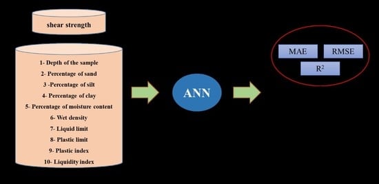
The prediction aptitude of an artificial neural network (ANN) is improved by incorporating two novel metaheuristic techniques, namely, the shuffled frog leaping algorithm (SFLA) and wind-driven optimization (WDO), for the purpose of soil shear strength (simply called shear strength) simulation. Soil information of the Trung Luong national expressway project (Vietnam) including depth of the sample (m), percentage of sand, percentage of silt, percentage of clay, percentage of moisture content, wet density (kg/m³), liquid limit (%), plastic limit (%), plastic index (%), liquidity index, and the shear strength (kPa) was collocated through a field survey. After constructing the hybrid ensembles of SFLA–ANN and WDO–ANN, both models were optimized in terms of complexity using a population-based trial-and error-scheme. The learning quality of the ANN was compared with both improved versions to examine the effect of the used metaheuristic techniques. In this phase, the training error dropped by 14.25% and 28.25% by applying the SFLA and WDO, respectively. This reflects a significant improvement in pattern recognition ability of the ANN. The results of the testing data revealed 25.57% and 39.25% decreases in generalization (i.e., testing) error. Moreover, the correlation between the measured and predicted shear strengths (i.e., the coefficient of determination) rose from 0.82 to 0.89 and 0.92, which indicates the efficiency of both SFLA and WDO metaheuristic techniques in optimizing the ANN.

1. Introduction

Soil shear strength is defined as the resistance of soil against shear stresses [1,2], which cause deformations or displacements in the soil mass [3]. Therefore, it is considered as one of the most crucial designing properties in geotechnical engineering. In the building sector, for example, having a reliable approximation of the shear strength helps foundation engineers to choose the type of foundation, as well as the necessity of subsoil improvement. It is also a very determinant factor for exploring soil problems like slope stability [4,5] and bearing capacity [6,7] in different conditions. Figure 1 illustrates an example of shear failures for strip footing subsoil and rainfall-induced landslide.

Like many other engineering problems, before the advent of soft computing approaches, the shear strength was investigated and predicted using statistical [8] and numerical methods [9,10,11,12]. Müller et al. [13] investigated uncertainty reduction in examining the undrained shear strength in clays using multivariate approaches. Garven and Vanapalli [14] provided a summary of 19 shear strength evaluative procedures consisting of six based on soil–water retention curve (SWRC), and 13 based on mathematical relationships. They also stated that the studied literature review highlighted the suitability of SWRC-based procedures for successful simulation of the shear strength. The shear strength can be affected by various soil factors like moisture content, plastic index, clay content, etc. [1]. Thus, implementing direct evaluative methods for exploring the relationship between the shear strength and its related parameters is relatively costly and complicated [15,16], and also there might lead to different results because of different stress states, stress histories, degrees of sampling disturbance, and strain rates [17]. Due to these difficulties, indirect methods are very popular in the field of geotechnical parameter evaluation [18,19,20].

In recent years, soft computing techniques gained increasing attention for simulating various geotechnical phenomena like slope stability [21,22,23,24]. As for the shear strength, many scholars showed the applicability of intelligent models. Chou et al. [25] showed the efficiency (correlation coefficient (R) = 0.89 and mean absolute percentage error (MAPE) = 3.27%) of machine learning for computing peak shear strength of discrete fiber-reinforced soils. Havaee et al. [26] used a multiple linear regression (MLR) model to predict the shear strength in the central part of Iran. Lee et al. [27] successfully employed an artificial neural network (ANN) for forecasting the unsaturated shear strength. Likewise, Wrzesiński et al. [28] used this tool for investigating the changes in undrained shear strength with respect to principal stress rotation. Besalatpour et al. [29] explored the prediction capability of an optimized support vector machine (SVM) for predicting the shear strength in Bazoft watershed, central Iran. The results were also compared with the multilayer perceptron (MLP) model. Regarding the R values of 0.98 and 0.52, along with mean absolute error (MAE) values of 0.17 and 0.81, the superiority of the SVM was derived. Moreover, the superiority of the ANN (to statistical models) was shown by Goktepe et al. [30] in analyzing the relationship between shear strength parameters and index properties of normally consolidated plastic clay.

The recent advances in metaheuristic science led to the proper optimization of different engineering parameters. Moreover, it was proven that synthesizing these algorithms with typical predictive models led to raising their accuracy through prevailing computational weaknesses [31,32,33]. In the field of shear strength analysis, well-known optimization algorithms such as the cuckoo search optimization (CSO), particle swarm optimization (PSO), and genetic algorithm (GA) were applied for the performance improvement of intelligent approaches of least-squares SVM, support vector regression (SVR), and adaptive neuro-fuzzy inference system (ANFIS) [6,34,35]. The findings of these studies demonstrated the better functioning of the metaheuristically reinforced models compared to regular versions. Despite the wide application of metaheuristic science in dealing with geotechnical problems, an appreciable gap of knowledge involves neural computing optimization for shear strength analysis, which was the motivation of the present research. Furthermore, regarding the necessity of seeking more efficient and state-of-the-art methods for the stated purpose, the second novelty of this paper involved employing hybrid evolutionary algorithms of the shuffled frog leaping algorithm (SFLA) and wind-driven optimization (WDO), which, according to the literature review, were not sufficiently used for this aim. These techniques contributed to the problem of shear strength modeling through fine-tuning the ANN computational parameters for analyzing the relationship between the shear strength and related factors.

2. Background of the Used Hybrid Science

2.1. Shuffled Frog Leaping Algorithm

Proposed by Eusuff and Lansey [36], the SFLA is a well-known optimization technique based on metaheuristic rules. An important reason for its popularity is combining the memetic algorithm and the PSO [37]. In addition, high convergence speed, as well as its simplicity, makes the SFLA an efficient global optimizer [38].

The population of this algorithm is composed of a set of frogs where each one indicates a possible solution to the defined problem. Mathematically, assuming p as the number of randomly produced individuals and D as the problem dimensions, the location of the i-th frog is defined as follows:

$$X_i=\left(x_{i1}, x_{i2}, \dots , x_{iD}\right).$$

(1)

The p is firstly divided into k memeplexes (the memeplexes contain a number of frogs with an identical structure). However, their adaptability is different. Based on the fitness of the frogs, they are lined in descending order. Then, the first frog of the first list contributes to the first memeplex, the second frog contributes to the next memeplex, and this process is kept until there are no more frogs to be assigned. Note that the first memeplex receives the k + 1-th frog at the end, and this process continues until all frogs contribute [39]. The explained procedure is depicted in Figure 2.

Next, the following equations are used to optimize the position of the bad frog ($X_{new}$):

$$S= \mathit{rand}\left(\right) \times \left(X_b- X_w\right),$$

(2)

$$X_{new}=X_w+S, S_{max}\ge S\ge -S_{max},$$

(3)

where $X_w$ and $X_b$ denote the worst and best positions of the frog in each memeplex, respectively. Also, rand () is a random value in the range [0, 1], and $S_{max}$ represents the frog’s maximum leap. In this sense, once the position of the bad frog is improved, $X_{new}$ replaces $X_w$; otherwise, $X_b$ gets replaced with the position of the elite frog ($X_g$). Then, $X_{new}$ is calculated. If the mentioned position is improved after that, $X_{new}$ replaces $X_w$; otherwise, a random value is assigned to $X_w$. This process continues until the defined number of updates is met. Finally, all individuals in all memeplexes are mixed and reordered in V memeplexes.

2.2. Wind-Driven Optimization

The name WDO represents a state-of-the-art metaheuristic technique suggested by Bayraktar et al. [40]. The initial idea was created for electromagnetic usage. The algorithm is inspired by air parcel movements in a multidimensional space. The four forces involved in this task are gravitational force (F_G), pressure gradient force (F_PG), Coriolis force (F_C), and frictional force (F_F). Mathematically, it is supposed that the air parcels are dimensionless and weightless to reduce the complexity of computation. Let ∇P and δV be the pressure gradient and finite volume of the air; then, Equation (4) expresses the force due to the pressure gradient. F_F (Equation (5)) aims to oppose the air movement triggered by F_PG. F_G (Equation (6)) pulls the parcels to the earth’s center from every dimension. Also, F_C (Equation (7)) attributes to the deflection in air parcel motions.

$$\overrightarrow{F_{PG}}= -\nabla P . \delta V,$$

(4)

$$\overrightarrow{F_F}= -\rho \alpha \overrightarrow{u},$$

(5)

$$\overrightarrow{F_G}= \rho . \delta V. \overrightarrow{g},$$

(6)

$$\overrightarrow{F_C}= -2 \theta \times \overrightarrow{u},$$

(7)

where g denotes the gravitational constant, $\rho$ represents the density of a short air parcel, $\overrightarrow{u}$ is the velocity vector of wind, $\alpha$ is a frictional coefficient, and $\theta$ symbolizes the earth’s rotation.

By considering the mentioned forces with the ideal gas equation, we obtain the following [41]:

$$\overrightarrow{\nabla u}= g+\left(-\nabla P.\frac{RT}{P_{cur}}\right)+\left(-\alpha \overrightarrow{u}\right)+\left(\frac{-2 \theta \times \overrightarrow{u}RT}{P_{cur}}\right),$$

(8)

Here, as the pressure increases, the velocity is adjusted because the air velocity depends on the pressure value. Consequently, with respect to the pressure rank, Equation (8) is modified. More clearly, based on the pressure, the parcels are ranked in descending order. In this sense, the velocity and position are updated using the following equations where i denotes the rank:

$$\overrightarrow{U_{new}}=\left(1- \alpha \right) {\overrightarrow{U}}_{cur}- g{x}_{cur}+\left(\left|1- \frac{1}{i}\right| . \left(x_{opt}- x_{cur}\right)RT\right)+\left(\frac{C . {\overrightarrow{U}}_{otherdirection}}{i}\right),$$

(9)

$$\overrightarrow{X_{new}}= \overrightarrow{X_{old}}+ \overrightarrow{U_{new}},$$

(10)

where ${\overrightarrow{U}}_{cur}$ and $\overrightarrow{U_{new}}$ represent the velocity of the current and coming iterations, x is the air parcel position, and $x_{opt}$ and $x_{cur}$ are the optimal and current positions. Meanwhile, ${\overrightarrow{U}}_{otherdirection}$ is equal to $\overrightarrow{F_C}$ and C = −2$RT$.

The explained updating process continues until one stopping criterion is met, like the set objective function (OF), or the number of repetitions. In the last step, the air parcel which has the lowest OF is found, and its corresponding parameters are used. More information can be found in previous studies [40,42,43].

3. Study Area and Data Collocation

The location of the study area is illustrated in Figure 3. It was the Trung Luong National Expressway section (with an overall length of nearly 140 km), a part of the Ho Chi Minh–Can Tho Expressway, Vietnam. The coordinates of the start and finish points of the proposed track are 10°25′ north (N) and 106°18′ east (E), and 10°41′ N and 106°34′ E, respectively. The project is anticipated to be completed at the end of 2019. With a designed speed of 120 km/h, the width of this road varies from 25.5 m (four-lane traffic in the first stage) to 33.0 m (six-lane traffic in the final stage) [34].

Extensive geotechnical field testing was carried out to obtain the soil information by sampling and implementing soil tests including the standard penetration test [44], vane shear test [45], and cone penetration test [46]. The data were collocated from 73 boreholes where their depths varied from 12.5 to 70.5 m.

For a total of 315 soil specimens, the information of 10 key factors, namely, depth of sample (DOP), percentage of sand, percentage of silt, percentage of clay, percentage of moisture content (MC), wet density (WD), liquid limit (LL), plastic limit (PL), plastic index (PI), and liquidity index (LI), was used to construct the input dataset, and the shear strength was considered to be the dependent variable. Figure 4 depicts the shear strength versus the independent factors. Also, the descriptive statistics of the used dataset are presented in

Table 1. Descriptive statistics of the used dataset.

Features	Descriptive Index
	Mean	SE *	Median	SD **	SV ***	Skewness	Minimum	Maximum
Depth of sample (m)	16.21	0.71	13.00	12.57	157.94	1.02	1.00	52.00
Sand (%)	8.40	0.73	2.40	13.04	169.92	1.85	0.00	57.30
Silt (%)	54.01	0.70	56.10	12.46	155.30	−0.30	20.00	83.70
Clay (%)	37.28	0.66	37.60	11.68	136.35	0.01	10.40	63.90
Moisture content (%)	48.47	1.35	49.90	23.90	571.41	0.12	17.10	90.30
Wet density (kg/m3)	1767.68	12.09	1690.00	214.60	46,054.17	0.09	1470.00	2150.00
Liquid limit (%)	54.47	0.84	54.90	14.89	221.65	−0.23	21.40	79.90
Plastic limit (%)	24.72	0.30	24.40	5.39	29.05	0.02	12.90	35.90
Plastic Index (%)	29.75	0.56	30.40	10.00	99.92	−0.27	6.60	49.70
Liquidity index	0.70	0.03	0.79	0.46	0.22	0.04	0.01	1.73
Shear strength (kPa)	42.12	1.76	20.81	31.31	980.23	0.55	8.27	130.00

* Standard error; ** standard deviation; *** sample variance.

.

4. Shear Strength Prediction Using Neural Hybrids of SFLA–ANN and WDO–ANN

4.1. Data Division and Preprocessing

Like other simulation methods, the development of intelligent models requires two sets of data, namely, training and testing samples [47]. The majority of data are specified to pattern analysis and training the models. The efficiency of the learning process is then evaluated by applying the network on unknown data (i.e., the testing samples). In other words, in this phase, the network predicts the shear strength for unseen soil conditions. The quality of testing results indicates the generalization capability of the model [48,49,50].

As mentioned, the dataset consisted of the information of 315 soil specimens. Out of those, 252 samples (i.e., 80% of the data) were selected for training the ANN, SFLA–ANN, and WDO–ANN models. Accordingly, the remaining 63 samples (i.e., 20% of the data) were devoted to the testing process. It is worth noting that the division of data was done based on a random selection process.

4.2. Initializing the MLP for Representing the ANN

Having a feed-forward hierarchical architecture, the multilayer perceptron (MLP) is the most commonly held notion of the ANNs [51,52]. In this study, an MLP neural network was used as the basic predictive model. It performed the prediction task by applying some weights and biases to the input variables within three or more layers. This work was carried out in the computational neurons within each layer. Although the number of neurons in the input and output layers was equal to the number of variables, this could be varied for the middle-layer neurons (also called “hidden neurons”). It is also one of the most influential factors in the performance of the MLP. Based on a trial-and-error process, different numbers of hidden neurons were tested, and the results showed that five of them constructed the best-fitted network. Moreover, the same process was used to determine the best values of other ANN parameters including learning rate, momentum factor, and learning cycles. These parameters were set to 1.0, 0.5, and 1000, respectively. Note that, their activation function was “tangent-sigmoid” (i.e., Tansig). This function is expressed as follows:

$$Tansig \left(x\right)= \frac{2}{1+ e^{-2x}}-1.$$

(11)

4.3. Defining Modeling Parameters

As explained, the SFLA and WDO algorithms function as optimization techniques that aim to find the best solution for a given problem. When these algorithms are synthesized with ANN, the problem is appropriately finding the best values of the weights (W) and biases (b) of each neuron through minimizing the difference between the actual and predicted shear strength. An objective function (OF) is defined here to measure the error of performance. The optimization process is implemented by a vast number of iterations. In general, the OF is expected to follow a downward trend during these iterations, which indicates an increase in accuracy. Notably, the OF in this study was considered to be the root-mean-square error (RMSE) which is defined in Section 4.5. Considering X as the input of the output neuron, the following mathematical relationships exist:

$$OF=RMSE \left(Output,Target\right),$$

(12)

$$Output=Tansig \left(\sum WX+b\right).$$

(13)

4.4. Hybridizing the ANN Using the SFLA and WDO

When it comes to metaheuristic algorithms, finding the best population size (PS) (i.e., the complexity) is an important task prior to running the main model. It is usually determined by a sensitivity analysis process. In this work, different values of PS were tested, including 10, 25, 50, 75, 100, 200, 300, 400, and 500. The best complexity was determined by evaluating the obtained OFs in the last iterations. The results are presented in Figure 5a. As can be seen, the lowest RMSE of the SFLA–ANN (10.4136) and WDO–ANN (9.3412) ensembles was obtained for the PSs of 10 and 300, respectively. The convergence curves of these networks are presented in Figure 5b,c.

4.5. Accuracy Assessment Criteria

Apart from the RMSE, MAE was also used to measure the error performance. Moreover, the coefficient of determination (R²) was used to measure the correlation between the observed and estimated shear strengths. Let Z_{i predicted} and Z_{i observed} be the estimated and observed shear strengths, and let $\overline{Z}$_observed be the average of Z_{i observed} values; then, Equations (14)–(16) express the formulations of the RMSE, MAE, and R², respectively.

$$RMSE=\sqrt{\frac{1}{N}{{\displaystyle \sum _{i=1}^N[(Z_{i observed}-Z_{i predicted})]}}^2},$$

(14)

$$MAE=\frac{1}{N}{\displaystyle \sum _{I=1}^N|Z_{i observed}-Z_{i predicted}|},$$

(15)

$$R^2=1-\frac{{\displaystyle \sum _{i=1}^N{(Z_{i predicted}-Z_{i observed})}^2}}{{\displaystyle \sum _{i=1}^N{(Z_{i observed}-{\overline{Z}}_{observed})}^2}},$$

(16)

where N is the number of data.

5. Results and Discussion

The prediction results in both training and testing phases are presented in this section. To this end, the products of the used models were compared with target values by using the mentioned accuracy criteria. As explained, the quality of the training results indicates the learning capability of the model. Figure 6 shows the results of this phase, in terms of the regular error (measured shear strength − predicted shear strength). As can be seen, the results of both reinforced ANNs were more accurate than the formal version. In detail, the RMSE experienced 11.33% (from 11.74 to 10.41) and 20.44% (from 11.74 to 9.34) reductions as the result of synthesizing the ANN with SFLA and WDO, respectively. The calculated MAEs confirmed these observations, as it was reduced by 14.25% (from 8.14 to 6.98) and 28.25% (from 8.14 to 5.84). In addition, referring to the obtained values of R² (0.85, 0.88, and 0.90), the superiority of the ensemble models was deduced. Therefore, both SFLA and WDO performed efficiently in enhancing the learning capability of the ANN.

The same criteria were applied to the outputs of the testing phase. In this phase, the RMSE of the ANN dropped from 15.11 to 12.20 (19.25%) and, more considerably, 11.13 (26.34%), by incorporation with the SFLA and WDO. As for the MAE, the decrease of this criterion from 11.26 to 8.38 (25.57%) and 6.84 (39.25%) indicated that the generalization accuracy of the ANN was increased. The comparison between the actual and predicted shear strengths is also shown in Figure 7. According to this figure, the hybrid models grasped a more reliable approximation of shear strength in comparison with ANN, especially for minimum and maximum values. These results are broadly discussed below.

The correlation of the testing results is depicted in Figure 8. Based on these figures, the products of the ANNs trained by the SFLA and WDO were better correlated with target shear strengths, compared to the ANN trained by the back-propagation learning method. This claim can be supported by the obtained values of R² of 0.8286, 0.8998, and 0.9258 (for all data), and 0.8732, 0.9187, and 0.9547 (for data inside 95% confidence limit boundaries), respectively, for the ANN, SFLA–ANN, and WDO–ANN. Notably, the observed shear strength ranged from 10.92 to 114.25, while the predicted values were in the ranges [3.40, 78.73], [7.09, 81.25], and [11.43, 86.41].

Due to the better performance (i.e., the higher accuracy) of the hybrid models, it was demonstrated that applying both SFLA and WDO is an effective way to increase the reliability of the ANN. From the comparison point of view, the results of the WDO algorithm were more promising than the SFLA. For more detail,

Table 2. Comparison between the SFLA—shuffled frog leaping algorithm and WDO—wind-driven optimization prediction for the maximum and minimum shear strengths values.

Type of Data	Observed Value (kPa)	Model Results		Relative Error (%)
		SFLA–ANN	WDO–ANN	SFLA–ANN	WDO–ANN
Minimum	8.27	12.55	13.01	51.79	57.33
	9.34	16.69	14.13	78.76	51.33
	9.34	15.92	14.88	70.40	59.26
	10.27	12.53	12.34	22.12	20.19
	10.27	15.29	11.51	48.96	12.15
Maximum	110.63	78.63	86.41	−28.93	−21.89
	111.55	72.08	72.78	−35.39	−34.76
	113.76	79.04	86.82	−30.51	−23.68
	114.25	77.97	79.65	−31.76	−30.28
	130.01	78.88	82.44	−39.32	−36.59

denotes the relative error (Equation (17)) calculated for five maximum and five minimum values of the shear strength dataset. In terms of minimum values, except for the lowest one (8.27), the relative errors of the WDO–ANN were lower than those of the SFLA–ANN. The most appreciable difference was related to the shear strength of 10.27. This value was predicted as 11.51 (around 12% error) by the WDO–ANN, while the SFLA–ANN had around 50% error in this sense. Evaluating the maximum shear strengths showed that all values were underestimated by both methods. Also, it was deduced that the relative errors of the WDO-based ensemble were lower than those of the SFLA-based ensemble. This points to the higher efficiency of the WDO for estimating the peak values of shear strength.

$$\mathrm{Relative} \mathrm{error} =(\frac{Z_{i predicted}-Z_{i observed}}{Z_{i observed}})\times 100.$$

(17)

In comparison with previous studies, the hybrid models of the present research outperformed the integration of least squares support vector machine (LSSVM) and the cuckoo search optimization (CSO), LSSVM–CSO, used by Bui et al. [34] for the same aim. More clearly, according to the obtained values of R², the prediction accuracy of both SFLA–ANN (0.89) and WDO–ANN (0.92) was higher than 0.885 in their study. However, the LSSVM was more successful in understanding the relationship between the shear strength and input factors (R² = 0.922 > 0.90). Similarly, the PSO–SVM used by Nhu et al. [6] predicted the shear strength less accurately (R² = 0.888) than both hybrid models of our study. More than 90% generalization accuracy of the WDO–ANN shows that it is a capable model to analyze and predict the shear strength for unseen soil conditions. In other words, it can be introduced as a promising alternative to laboratory and traditional shear strength evaluative methods. Hence, the ruling formulation of this model was extracted, and it is presented in Equation (18) for use as an efficient neural–mathematical solution to the problem of shear strength modeling. This formula, as well as Equation (19), was derived using the weights and biases of the MLP which were optimized by the WDO algorithms. More specifically, Equation (18) was extracted from the output neuron of the MLP network, which was fed by A, B, …, E. These middle parameters represent the outputs of the hidden neurons. As can be seen, the activation function of Tansig was applied to these outputs.

Shear strength_WDO-ANN = −0.7757 × A + 0.4752 × B − 0.7565 × C − 0.5395 × D + 0.2687× E − 0.4902.

(18)

$$\left[\begin{array}{c}\mathrm{A}\\ \mathrm{B}\\ \mathrm{C}\\ \mathrm{D}\\ \mathrm{E}\end{array}\right]=\mathit{Tansig}\left(\right(\left[\begin{array}{cccccccccc}0.4182& 0.7457& -0.0538& 0.2524& 1.0098& -0.4615& 0.0951& 0.2266& -0.7045& 0.3425\\ 0.8331& -0.2381& -0.2327& -0.3187& -0.6103& 0.2087& -0.1710& 0.7667& 0.2941& 0.8237\\ 0.5166& 0.2242& -0.8520& -0.7931& 0.0367& 0.7373& 0.3965& -0.0099& -0.0890& 0.5675\\ -0.7339& 0.8113& -0.6531& 0.1438& -0.0184& -0.5871& 0.3188& -0.2853& -0.0649& 0.7266\\ 0.7275& 0.5602& -0.1922& 0.4500& 0.7937& 0.1034& 0.4448& -0.5363& 0.6534& 0.2622\end{array}\right]\left[\begin{array}{c}\mathrm{DOS}\\ \mathrm{Sand}\\ \mathrm{Silt}\\ \mathrm{Clay}\\ \mathrm{MC}\\ \mathrm{WD}\\ \mathrm{LL}\\ \mathrm{PL}\\ \mathrm{PI}\\ \mathrm{LI}\end{array}\right])+[\begin{array}{c}-1.6445\\ -0.8222\\ 0.0000\\ -0.8222\\ 1.6445\end{array}\left]\right).$$

(19)

6. Concluding Remarks

The robustness of the shuffled frog leaping algorithm and wind-driven optimization techniques for optimizing the performance of a neural network was evaluated in this paper. The models were applied to an important engineering problem, namely, soil shear strength prediction, for a real-world construction project. Although the ANN showed good accuracy in predicting the shear strength, it was shown that the computational drawbacks of this model can be addressed by synthesizing it with both the SFLA and the WDO algorithms. Due to the existing difficulties of traditional shear strength evaluative methods (e.g., laboratory tests and analytical approaches), as well as the high competency of the studied tools, both ensemble models of this paper can be used as inexpensive yet accurate alternatives for simulating the shear strength. In this regard, the neural–metaheuristic formula of the most successful model (i.e., the WDO) was extracted and presented.

References

- Das, B.M.; Sobhan, K. Principles of Geotechnical Engineering; Cengage Learning: Boston, MA, USA, 2013. [Google Scholar]
- Terzaghi, K.; Peck, R.B.; Mesri, G. Soil Mechanics in Engineering Practice; John Wiley & Sons: New York, NY, USA, 1996. [Google Scholar]
- Hundy, L.C. Plant Growth and Soil Shear Strength in Relation to Soil Properties and Hydro-Edaphic Characteristics of Restored Louisiana Salt Marshes. Master’s Thesis, University of Louisiana at Lafayette, Ann Arbor, MI, USA, 2015. [Google Scholar]
- Stark, T.D.; Choi, H.; McCone, S. Drained shear strength parameters for analysis of landslides. J. Geotech. Geoenviron. Eng. 2005, 131, 575–588. [Google Scholar] [CrossRef]
- Collins, B.D.; Znidarcic, D. Stability analyses of rainfall induced landslides. J. Geotech. Geoenviron. Eng. 2004, 130, 362–372. [Google Scholar] [CrossRef]
- Nhu, V.-H.; Hoang, N.-D.; Duong, V.-B.; Vu, H.-D.; Bui, D.T. A hybrid computational intelligence approach for predicting soil shear strength for urban housing construction: A case study at Vinhomes Imperia project, Hai Phong city (Vietnam). Eng. Comput. 2019, 1–14. [Google Scholar] [CrossRef]
- Popescu, R.; Deodatis, G.; Nobahar, A. Effects of random heterogeneity of soil properties on bearing capacity. Probab. Eng. Mech. 2005, 20, 324–341. [Google Scholar] [CrossRef]
- Houlsby, N.; Houlsby, G. Statistical fitting of undrained strength data. Géotechnique 2013, 63, 1253. [Google Scholar] [CrossRef]
- Motaghedi, H.; Eslami, A. Analytical approach for determination of soil shear strength parameters from CPT and CPTu data. Arab. J. Sci. Eng. 2014, 39, 4363–4376. [Google Scholar] [CrossRef]
- Vanapalli, S.; Fredlund, D. Empirical Procedures to predict the shear strength of unsaturated soils. In Proceedings of the Eleventh Asian Regional Conference on Soil Mechanics and Geotechnical Engineering, Seoul, Korea, 16–20 August 1999; pp. 93–96. [Google Scholar]
- Motaghedi, H.; Armaghani, D.J. New method for estimation of soil shear strength parameters using results of piezocone. Measurement 2016, 77, 132–142. [Google Scholar] [CrossRef]
- Gao, W.; Wang, W.; Dimitrov, D.; Wang, Y. Nano properties analysis via fourth multiplicative ABC indicator calculating. Arab. J. Chem. 2018, 11, 793–801. [Google Scholar] [CrossRef]
- Müller, R.; Larsson, S.; Spross, J. Extended multivariate approach for uncertainty reduction in the assessment of undrained shear strength in clays. Can. Geotech. J. 2013, 51, 231–245. [Google Scholar] [CrossRef]
- Garven, E.; Vanapalli, S. Evaluation of empirical procedures for predicting the shear strength of unsaturated soils. In Unsaturated Soils 2006; ASCE Press: Reston, VA, USA, 2006; pp. 2570–2592. [Google Scholar]
- Rassam, D.W.; Williams, D.J. A relationship describing the shear strength of unsaturated soils. Can. Geotech. J. 1999, 36, 363–368. [Google Scholar] [CrossRef]
- Gan, J.; Fredlund, D.; Rahardjo, H. Determination of the shear strength parameters of an unsaturated soil using the direct shear test. Can. Geotech. J. 1988, 25, 500–510. [Google Scholar] [CrossRef]
- Ching, J.; Phoon, K.-K. Multivariate distribution for undrained shear strengths under various test procedures. Can. Geotech. J. 2013, 50, 907–923. [Google Scholar] [CrossRef]
- Moavenian, M.; Nazem, M.; Carter, J.; Randolph, M. Numerical analysis of penetrometers free-falling into soil with shear strength increasing linearly with depth. Comput. Geotech. 2016, 72, 57–66. [Google Scholar] [CrossRef]
- Kulhawy, F.H.; Mayne, P.W. Manual on Estimating Soil Properties for Foundation Design; Electric Power Research Inst., Cornell Univ.: Palo Alto, CA, USA, 1990. [Google Scholar]
- Gao, W.; Wu, H.; Siddiqui, M.K.; Baig, A.Q. Study of biological networks using graph theory. Saudi J. Biol. Sci. 2018, 25, 1212–1219. [Google Scholar] [CrossRef] [PubMed]
- Moayedi, H.; Hayati, S. Applicability of a CPT-based neural network solution in predicting load-settlement responses of bored pile. Int. J. Geomech. 2018, 18. [Google Scholar] [CrossRef]
- Bui, D.T.; Tuan, T.A.; Klempe, H.; Pradhan, B.; Revhaug, I. Spatial prediction models for shallow landslide hazards: A comparative assessment of the efficacy of support vector machines, artificial neural networks, kernel logistic regression, and logistic model tree. Landslides 2016, 13, 361–378. [Google Scholar]
- Gao, W.; Guirao, J.L.G.; Abdel-Aty, M.; Xi, W. An independent set degree condition for fractional critical deleted graphs. Discret. Contin. Dyn. Syst. 2019, 12, 877–886. [Google Scholar] [CrossRef] [Green Version]
- Gao, W.; Guirao, J.L.G.; Basavanagoud, B.; Wu, J. Partial multi-dividing ontology learning algorithm. Inf. Sci. 2018, 467, 35–58. [Google Scholar] [CrossRef]
- Chou, J.-S.; Yang, K.-H.; Lin, J.-Y. Peak shear strength of discrete fiber-reinforced soils computed by machine learning and metaensemble methods. J. Comput. Civ. Eng. 2016, 30, 04016036. [Google Scholar] [CrossRef] [Green Version]
- Havaee, S.; Mosaddeghi, M.; Ayoubi, S. In situ surface shear strength as affected by soil characteristics and land use in calcareous soils of central Iran. Geoderma 2015, 237, 137–148. [Google Scholar] [CrossRef]
- Lee, S.; Lee, S.R.; Kim, Y. An approach to estimate unsaturated shear strength using artificial neural network and hyperbolic formulation. Comput. Geotech. 2003, 30, 489–503. [Google Scholar] [CrossRef]
- Wrzesiński, G.; Sulewska, M.; Lechowicz, Z. Evaluation of the Change in Undrained Shear Strength in Cohesive Soils due to Principal Stress Rotation Using an Artificial Neural Network. Appl. Sci. 2018, 8, 781. [Google Scholar] [CrossRef] [Green Version]
- Besalatpour, A.; Hajabbasi, M.; Ayoubi, S.; Gharipour, A.; Jazi, A. Prediction of soil physical properties by optimized support vector machines. Int. Agrophys. 2012, 26, 109–115. [Google Scholar] [CrossRef] [Green Version]
- Goktepe, A.B.; Altun, S.; Altintas, G.; Tan, O. Shear strength estimation of plastic clays with statistical and neural approaches. Build. Environ. 2008, 43, 849–860. [Google Scholar] [CrossRef]
- Moayedi, H.; Osouli, A.; Nguyen, H.; Rashid, A.S.A. A novel Harris hawks’ optimization and k-fold cross-validation predicting slope stability. Eng. Comput. 2019, 1–11. [Google Scholar] [CrossRef]
- Moayedi, H.; Mehrabi, M.; Kalantar, B.; Abdullahi Mu’azu, M.; Rashid, A.S.; Foong, L.K.; Nguyen, H. Novel hybrids of adaptive neuro-fuzzy inference system (ANFIS) with several metaheuristic algorithms for spatial susceptibility assessment of seismic-induced landslide. Geomat. Nat. Hazards Risk 2019, 10, 1879–1911. [Google Scholar] [CrossRef] [Green Version]
- Gao, W.; Dimitrov, D.; Abdo, H. Tight independent set neighborhood union condition for fractional critical deleted graphs and ID deleted graphs. Discret. Contin. Dyn. Syst. 2018, 12, 711–721. [Google Scholar] [CrossRef] [Green Version]
- Bui, D.T.; Hoang, N.-D.; Nhu, V.-H. A swarm intelligence-based machine learning approach for predicting soil shear strength for road construction: A case study at Trung Luong National Expressway Project (Vietnam). Eng. Comput. 2019, 35, 955–965. [Google Scholar]
- Pham, B.T.; Hoang, T.-A.; Nguyen, D.-M.; Bui, D.T. Prediction of shear strength of soft soil using machine learning methods. Catena 2018, 166, 181–191. [Google Scholar] [CrossRef]
- Eusuff, M.M.; Lansey, K.E. Optimization of water distribution network design using the shuffled frog leaping algorithm. J. Water Resour. Plan. Manag. 2003, 129, 210–225. [Google Scholar] [CrossRef]
- Liping, Z.; Weiwei, W.; Yi, H.; Yefeng, X.; Yixian, C. Application of shuffled frog leaping algorithm to an uncapacitated SLLS problem. AASRI Procedia 2012, 1, 226–231. [Google Scholar] [CrossRef]
- Zhang, X.; Zhang, Y.; Shi, Y.; Zhao, L.; Zou, C. Power control algorithm in cognitive radio system based on modified shuffled frog leaping algorithm. AEU-Int. J. Electron. Commun. 2012, 66, 448–454. [Google Scholar] [CrossRef]
- Chen, W.; Panahi, M.; Tsangaratos, P.; Shahabi, H.; Ilia, I.; Panahi, S.; Li, S.; Jaafari, A.; Ahmad, B.B. Applying population-based evolutionary algorithms and a neuro-fuzzy system for modeling landslide susceptibility. Catena 2019, 172, 212–231. [Google Scholar] [CrossRef]
- Bayraktar, Z.; Komurcu, M.; Werner, D.H. Wind Driven Optimization (WDO): A novel nature-inspired optimization algorithm and its application to electromagnetics. In Proceedings of the 2010 IEEE Antennas and Propagation Society International Symposium, Toronto, ON, Canada, 11–17 July 2010; pp. 1–4. [Google Scholar]
- Derick, M.; Rani, C.; Rajesh, M.; Farrag, M.; Wang, Y.; Busawon, K. An improved optimization technique for estimation of solar photovoltaic parameters. Sol. Energy 2017, 157, 116–124. [Google Scholar] [CrossRef]
- Bayraktar, Z.; Komurcu, M.; Bossard, J.A.; Werner, D.H. The wind driven optimization technique and its application in electromagnetics. IEEE Trans. Antennas Propag. 2013, 61, 2745–2757. [Google Scholar] [CrossRef]
- Bhandari, A.K.; Singh, V.K.; Kumar, A.; Singh, G.K. Cuckoo search algorithm and wind driven optimization based study of satellite image segmentation for multilevel thresholding using Kapur’s entropy. Expert Syst. Appl. 2014, 41, 3538–3560. [Google Scholar] [CrossRef]
- Clayton, C.R. The Standard Penetration Test (SPT): Methods and Use; Construction Industry Research and Information Association: London, UK, 1995. [Google Scholar]
- ASTM. Standard Test Method for Laboratory Miniature Vane Shear Test for Saturated Fine-Grained Clayey Soil; ASTM International: West Conshohocken, PA, USA, 2016. [Google Scholar]
- Schmertmann, J.H.; United States Federal Highway Administration. Guidelines for Cone Penetration Test: Performance and Design; United States Federal Highway Administration: Washington, DC, USA, 1978.
- Moayedi, H.; Mehrabi, M.; Mosallanezhad, M.; Rashid, A.S.A.; Pradhan, B. Modification of landslide susceptibility mapping using optimized PSO-ANN technique. Eng. Comput. 2018, 35, 1–18. [Google Scholar] [CrossRef]
- Bui, D.T.; Ghareh, S.; Moayedi, H.; Nguyen, H. Fine-tuning of neural computing using whale optimization algorithm for predicting compressive strength of concrete. Eng. Comput. 2019, 1–12. [Google Scholar] [CrossRef]
- Moayedi, H.; Bui, D.T.; Gör, M.; Pradhan, B.; Jaafari, A. The feasibility of three prediction techniques of the artificial neural network, adaptive neuro-fuzzy inference system, and hybrid particle swarm optimization for assessing the safety factor of cohesive slopes. ISPRS Int. J. Geo-Inf. 2019, 8, 391. [Google Scholar] [CrossRef] [Green Version]
- Bui, D.T.; Moayedi, H.; Gör, M.; Jaafari, A.; Foong, L.K. Predicting slope stability failure through machine learning paradigms. ISPRS Int. J. Geo-Inf. 2019, 8, 395. [Google Scholar] [CrossRef] [Green Version]
- Kim, C.M.; Parnichkun, M. MLP, ANFIS, and GRNN based real-time coagulant dosage determination and accuracy comparison using full-scale data of a water treatment plant. J. Water Supply Res. Technol. 2016, 66, 49–61. [Google Scholar] [CrossRef]
- Örnek, M.N.; Kahramanli, H. Determining the Carrot Volume via Radius and Length Using ANN. Int. J. Intell. Syst. Appl. Eng. 2018, 6, 165–169. [Google Scholar] [CrossRef] [Green Version]
Figure 1.
Failure mechanism of (a) Bearing capacity failure, and (b) Slope failure example.
Figure 2.
Leaping procedure of the shuffled frog leaping algorithm (SFLA) algorithm.
Figure 3.
Location of the studied track.
Figure 4.
The relationship between shear strength and the input variables; (a): depth of sample, (b): percentage of sand, (c): percentage of silt, (d): percentage of clay, (e): percentage of moisture content, (f): wet density, (g): liquid limit, (h): plastic limit, (i): plastic index, and (j): liquidity index.
Figure 5.
(a) The results of the executed sensitivity analysis; (b,c) the convergence curves of the elite SFLA–artificial neural network (ANN) and wind-driven optimization (WDO)–ANN, respectively.
Figure 6.
The training results of the implemented (a) typical ANN, (b) SFLA–ANN, and (c) WDO–ANN.
Figure 7.
The testing results of the implemented (a) typical ANN, (b) SFLA–ANN, and (c) WDO–ANN.
Figure 8.
The correlation between the measured and predicted shear strengths in the testing phases; (a) R2 = 0.8286, (b) R2 = 0.8998, (c) R2 = 0.9258.