Experimental and CFD Investigation into Using Inverted U-Tube for Gas Entrainment

Abstract

An experimental and numerical study is presented in the current work for gas entrainment using an inverted vertical U-tube. Water flows vertically up in an inverted U-tube which creates a low-pressure region in the tube upper portion. This low-pressure region can be used to extract gases by connecting it to a branch pipe. The extracted gases considered in this work are a mixture of air and water vapor. The water vapor from the side branch pipe is mixed with the flowing water under the siphon effect. This results in a progressive water vapor condensation as the mixture proceeds towards the exit due to an increase in vapor partial pressure. The air is drawn by inertia to be released out at the tube lower exit of the inverted U-pipe. The current study deals with these complicated flow behaviors due to the mixing undergoing condensation. A test rig is designed for experimentally studying the behavior of water flow in an inverted U-tube where the air is mixed with the flowing water at the top region of this tube. The CFD computations are accomplished for a side gas mixture with volume fractions up to 0.7 with water vapor mass fractions in this mixture to be 0.1–0.5. The tested water mass flow rates in the main tube are 2, 4, 6, 8 kg/s to account for all possible flow mass ratios. The CFD computations are validated with water and air two phase flow with the measurements of both the experiments of the current research and the literature. The present results reveal that slightly raising the water mass flow rate at a constant side mixture mass ratio produces a reduced generated pressure in the upper tube part. This is attributed to extra water vapor condensation taking place rapidly by increasing the water flow rate in the tube upper part. Furthermore, the turbulence quantities begin to break down at a side mixture volume fraction of 0.55 with water and air mass flow rates of 2 kg/s and 0.002 kg/s, respectively. On the other side, raising the air mass flow rate at the higher values of water vapor and water mass flow rates breaks the generated vacuum pressure and turbulence due to entrainment. Moreover, this proposed framework can produce a lower static pressure, reaching 55.1 kPa, which makes it attractive for gas extraction. This new technique presents innovative usage with less consumable energy for extracting gases in engineering equipment.

1. Introduction

Few engineering and medical applications need evacuated cavities during certain manufacturing and testing processes. These evacuated cavities may contain a variety of gases and liquids. So, the continuous removal of these undesired fluids and maintenance of the required evacuated cavities at a specific pressure becomes mandatory for these applications. The most used devices for venting these gases are categorized as a steam trap, liquid ring, vacuum pumps, manual valve, automatic valve and steam ejector. All these devices consume a considerable amount of energy to accomplish their duties. The use of an inverted U-tube is an innovative method for entraining such gases, which may lead to the consumption of less energy [1]. When water flows up in an inverted U-tube, it produces a low-pressure region at its upper part. This produces a low-pressure region, which can be exploited to draw gases from the required cavity by connecting the top of the inverted U-tube to the cavity through a side pipe. In the present paper, two-phase flow (water and gas) and three components (water liquid, air and water vapor) are considered in the proposed CFD computations. One of the most important pieces of equipment working under vacuum is the steam condenser of the steam power plant. The main function of the steam condenser, besides steam condensation, is to preserve the generated operational vacuum by evacuating the gases in the cycle. Currently, steam power plants share the largest percentage of electricity generation worldwide [2,3].

As commonly known in a condenser, the volume fractions of air, vapor, and water change rapidly, and this complicated behavior has a significant impact on plant efficiency. Water vapor can be taken out of the condenser cavity through condensation and it is pumped back to the water feeding system of the plant boiler. The non-condensable gas is mainly air that has leaked into the plant turbine and condenser, which are working below the atmospheric pressure or it comprises air and non-condensable gases released from the plant working fluid. Furthermore, these non-condensable gases may also be formed by water decomposition. For efficient plant operation, these gases are extracted out of the condenser cavity to avoid increasing the condenser operating pressure. Raising the condenser operating pressure diminishes the steam turbine output power. Additionally, these gases severely reduce the heat transfer rates in the condenser by the covering wrap of its tubes. Furthermore, the oxygen content raises the tube corrosiveness in the condenser, which lowers the condenser’s operational life. So, these gases should be evacuated continuously for better operation and longer life of the steam condenser [4,5,6].

Few experiments consider the two-phase flow of steam condensation with the presence of gas in vertical tubes [7,8,9]. The main finding of these experiments was that raising both the gas mass fraction and the inlet properties reduced the heat transfer rate. Additionally, the local heat transfer was measured in the case of steam only and steam mixed with helium and air. The obtained temperature profiles for the considered cases provided a reasonable way of validating the proposed numerical model. The CFD computations of condensation in the existence of gases encountered some implementing difficulties but the resulted CFD flow profiles helped to investigate the physical mechanisms due to condensation. The effect of non-condensing gases on the steam condenser performance is presented theoretically by Strušnik et al. [10]. In their study, the steam ejector pump system is modeled by monitoring the gas extraction. Optimizing the steam ejector pump geometry was recommended for enhancing plant efficiency [10]. Strušnik et al. [11] made a comparative study for the power consumptions in the case of using the ejector and electric vacuum pump. They presented an economic analysis and operating costs guidelines for the appropriate selection of the condenser evacuating system in the steam power plant. It was found that the considered ejector is more consuming for the plant energy, as compared to the liquid ring vacuum pump. The condensation of steam with the existence of non-condensing gas was studied in [12,13]. They explored that the existence of the non-condensing gases severely reduced the heat transfer coefficient in the steam condenser. A hybrid system for gas extraction in the plant condenser was studied by Kapooria et al. [4]. In this hybrid system, a steam ejector integrated with a liquid ring vacuum pump was utilized. This proposed hybrid system was able to generate more vacuum in the steam condenser, while an observed increase in energy consumption was recorded.

Significant attention has been directed toward the complicated air and water flow patterns and their application in the steam condenser. In this regard, Yao et al. [14] studied numerically the two-phase flow of air/water in a small horizontal pipe. The obtained CFD results had an acceptable agreement with the considered experimental data and the CFD simulation accurately predicted the flow structures. The noticed small discrepancies between the experimental data and the CFD results may be attributed to the requirement for the full three-dimensional CFD simulations. In the same way, Juggurnath et al. [15] numerically presented the various two-phase flow profiles created in an inclined tube. They considered the effect of both surface tension and gravitational forces on the generated flow patterns. The air/water flow in a horizontal pipe was investigated numerically by Vásquez et al. [16]. Different multiphase flow models were used for obtaining the flow patterns and the proposed CFD model was validated. The validation showed a reasonable agreement with slight deviations. Seven experimental facilities for the air and water co-current flow in sloping pipes were presented by Pothof and Clemens [17]. A CFD geometrical and operational analysis for preventing the air accumulation in the tube was proposed. Panella [18] numerically and experimentally predicted the air and water flow in pipes. In this study, a framework for mixing air and water in the tube is fabricated. A circulating pump was utilized for controlling the water mass flow rate. This study revealed good validation in a wide range of data. Air and water two-phase flow in a tube with gas separator was presented by Afolabi and Lee [19]. This study ensured the ability of CFD models to accurately predict the behavior of the two-phase flow. Besides, the computational results had a good validation with the experiments.

The objective of the present work is to numerically capture the two-phase flow patterns in the inverted U-tube when mixing water with a side mixture of air and water vapor. Furthermore, the required flow conditions and operational parameters for using the inverted U-tube for the side entrainment of the air-water vapor mixture will be determined. Additionally, a reduced scale experimental test rig is fabricated to validate the present CFD results.

2. Experimental Setup

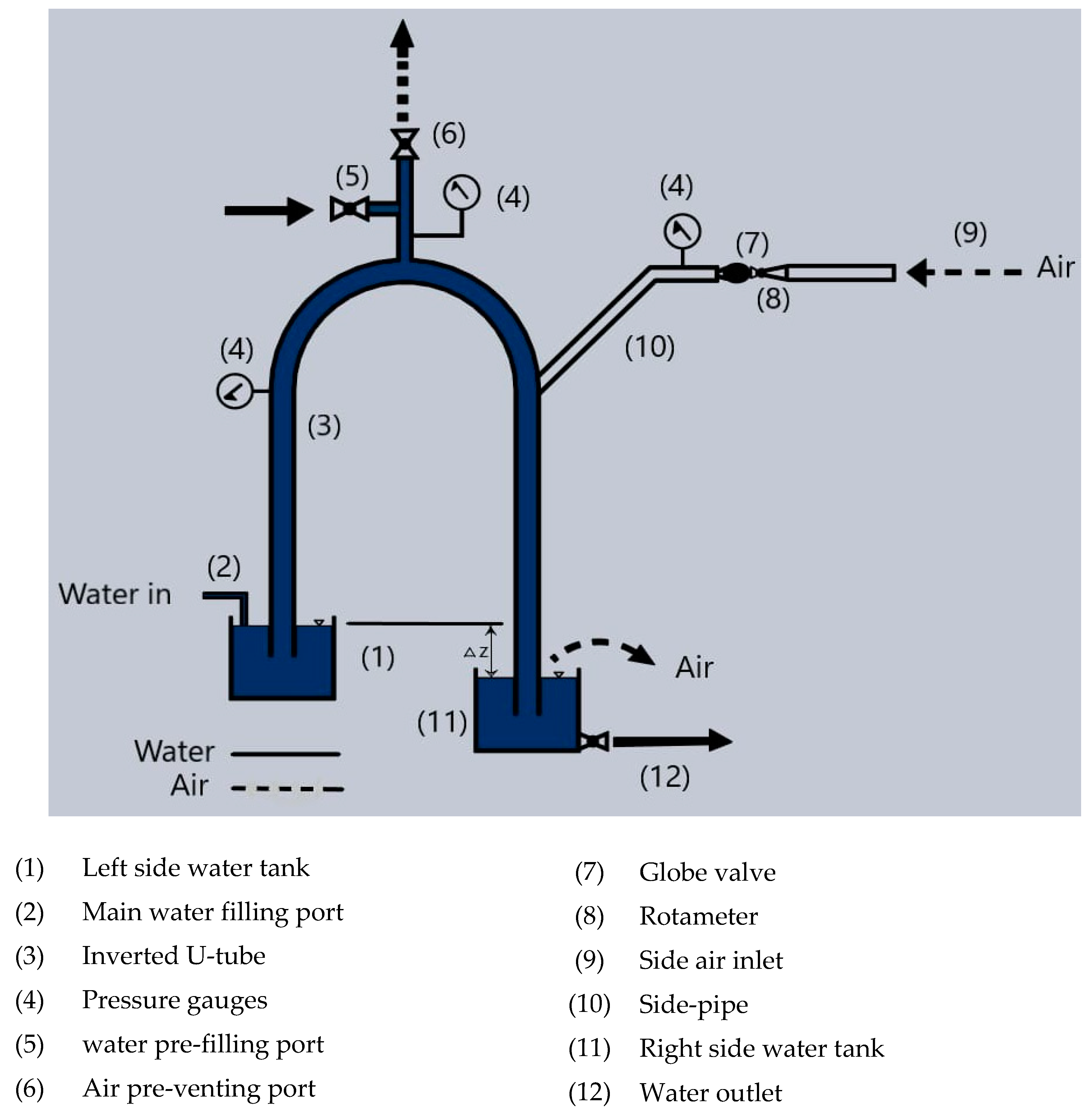
An experimental setup is fabricated to disclose the siphon flow characteristics with side air entrainment in the inverted U-tube. The experimental test rig with half scaled dimensions, compared to the CFD model dimensions, is fabricated. The experimental set up comprises two tanks with a water elevation difference of ΔZ—see Figure 1. An inverted U-tube of 2.54 cm inner diameter, with its inlets immersed into the two water tanks, is utilized. The water levels in the tanks are changeable by lowering/lifting the right-side tank. The main filling port (2) in the left side tank and a water exit port in the right-side tank (12) is used to maintain the water levels between the two tanks constant during measurements. Bourdon pressure gauges (4) are utilized to measure the flow pressure around the system. The flowing water through the inverted U-tube is measured by using a calibrated tank and stopwatch while the side air is measured by using a variable area rotameter (7). The rotameter has a full-scale accuracy/repeatability of 6/2%. The rotameter has a variable flow area valve (8) to control the inlet air flow rate (9). The siphon flow generation is one of the tricky points before measurements. The pre-filling port (5) is used to fill the whole system with water while the air venting port (6) is used to release the air from the system cavity. The inverted U-tube inlets in the right- and left-side tanks are blocked during this system pre-filling by using manual valves.

Once the whole system is full of water and free of air, the inverted U-tube inlets in the right- and left-side tanks are unblocked while maintaining the water pre-filling port (5) opened to help initiate the siphon flow for a while. Reaching a steady siphon flow is the main task that should be performed first. Then, the desired water elevation difference between the left and right tanks is obtained and kept constant. The water flow rate is measured before and after side air enters the system at the same ΔZ. The air flow rate is changeable by using the variable area valve (8), which is also used to close the side pipe during the siphon flow initiation. The water level difference between the two tanks can be changed by adjusting the side air entrainment and the experiments are repeated for different flow conditions.

3. Computational Model

The two-phase model is a set of equations and mathematical relations that are used to describe the phase’s motion and interactions. The most commonly utilized two-phase models in the literature are homogeneous, drift flux and separated flow models [20,21,22,23,24,25]. The homogeneous model is less complicated and can be applied to many complex two-phase flows with good accuracy. The homogeneous model is represented by the mixture two-phase model in CFD computations, as will be discussed later in this paper. In homogenous models, the average properties for the flow variables are considered in the calculations and the relative motion between phases can be accurately calculated [20,26]. In addition, the homogenous model is easy to implement as its governing equations are close to the single-phase flow equations. In the present study, the mixture model for calculating the two-phase flow variables in the inverted U-tube is utilized.

Figure 2 shows the CFD model with its boundary conditions. In the proposed work, the siphon flow generated by water flowing up in an inverted U-tube creates a vacuum in the tube upper region. This vacuum region can be connected by a side pipe to extract a mixture of air and water vapor from the equipment cavity, the equipment cavity is not shown in this figure. The equipment cavity is considered the steam condenser in the present case. This results in mixing the water with the induced side mixture of air and water vapor. This mixing will cause the water vapor condensation while all the flow mixture will continue flowing down due to flow inertia and gravity. At the lower outlet of the inverted U-tube, the air is released to the environment while water is re-circulated through the inverted U-tube. Furthermore, a variable speed circulating pump is used to transfer the water between the two tanks at the inlet and outlet of the inverted U-tube (the pump is not shown in the figure). Additionally, the hydrostatic head difference between the water surfaces in both tanks can be altered to control the water mass flow rate. The considered tube has low maintenance and operational cost, which makes it more favorable compared to the other energy consuming systems, i.e., water ring pump and steam ejector [27].

3.1. Governing Equations

Steady-state three dimensional CFD computations were performed for the considered geometry shown in Figure 2. Differential equations governing the fluid flow are given as [28,29].

$$\Delta \left(\mathsf{\rho }\mathrm{u}\right) =0$$

(1)

$$\Delta \left(\mathsf{\rho }\mathrm{u} \mathrm{u}\right)=-\frac{\partial \mathrm{p}}{\partial \mathrm{x}}+\Delta \left(\mathsf{\mu } \mathrm{grad} \mathrm{u}\right)+\left[-\frac{\partial \overline{\mathsf{\rho }{{\mathrm{u}}^{\prime }}^2}}{\partial \mathrm{x}}-\frac{\partial \overline{\mathsf{\rho }{\mathrm{u}}^{\prime } {\mathrm{v}}^{\prime }}}{\partial \mathrm{y}}-\frac{\partial \overline{\mathsf{\rho }{\mathrm{u}}^{\prime } {\mathrm{w}}^{\prime }}}{\partial \mathrm{z}}\right]$$

(2)

$$\Delta \left(\mathsf{\rho }\mathrm{u} \mathrm{v} \right)=-\frac{\partial \mathrm{p}}{\partial \mathrm{y}}+\Delta \left(\mathsf{\mu } \mathrm{grad} \mathrm{v}\right)+\left[-\frac{\partial \overline{\mathsf{\rho } {\mathrm{u}}^{\prime } {\mathrm{v}}^{\prime }}}{\partial \mathrm{x}}-\frac{\partial \overline{\mathsf{\rho } {{\mathrm{v}}^{\prime }}^2}}{\partial \mathrm{y}}-\frac{\partial \overline{\mathsf{\rho } {\mathrm{v}}^{\prime } {\mathrm{w}}^{\prime }}}{\partial \mathrm{z}}\right]$$

(3)

$$\Delta \left(\mathsf{\rho }\mathrm{u} \mathrm{w} \right)=-\frac{\partial \mathrm{p}}{\partial \mathrm{z}}+\Delta \left(\mathsf{\mu } \mathrm{grad} \mathrm{w}\right)+\left[-\frac{\partial \overline{\mathsf{\rho }{\mathrm{u}}^{\prime } {\mathrm{w}}^{\prime }}}{\partial \mathrm{x}}-\frac{\partial \overline{\mathsf{\rho }{\mathrm{v}}^{\prime } {\mathrm{w}}^{\prime }}}{\partial \mathrm{y}}-\frac{\partial \overline{\mathsf{\rho } {{\mathrm{w}}^{\prime }}^2}}{\partial \mathrm{z}}\right]$$

(4)

The energy equation can be found as follows to consider the heat transfer, as in the current study.

$$\Delta \left(\mathsf{\rho }\mathrm{Iu}\right)=\Delta \left(\mathrm{k} \mathrm{grad} \mathrm{T}\right)+\mathsf{\Phi }+\left[-\frac{\partial \overline{\mathsf{\rho } {\mathrm{u}}^{\prime } {\mathrm{I}}^{\prime }}}{\partial \mathrm{x}}-\frac{\partial \overline{\mathsf{\rho } {\mathrm{v}}^{\prime } {\mathrm{I}}^{\prime }}}{\partial \mathrm{y}}-\frac{\partial \overline{\mathsf{\rho } {\mathrm{w}}^{\prime } {\mathrm{I}}^{\prime }}}{\partial \mathrm{z}}\right]$$

(5)

I is the total energy, $\mathrm{I}=\mathrm{h}-\frac{p}{\rho }+\frac{\left(u^2+v^2\right)}{2}$, while $\mathsf{\Phi }$ is the function of dissipation. $\mathrm{h}$ is taken to be the sensible enthalpy where $\mathrm{h}={\displaystyle \sum }_{\mathrm{i}}{\mathrm{Y}}_{\mathrm{i}}{\mathrm{h}}_{\mathrm{i}}$ and ${\mathrm{h}}_{\mathrm{i}}={{\displaystyle \int }}_{{\mathrm{T}}_{\mathrm{ref}}}^{\mathrm{T}}{\mathrm{C}}_{\mathrm{pi}}\mathrm{dT}$. ${\mathrm{T}}_{\mathrm{ref}}$ is the reference temperature and it is equal to 298.2 K.

3.2. Realizable $k-\epsilon$ Model

In the present study, the realizable $\mathit{k}-\mathit{\epsilon }$ model in the mixture form is utilized for computing the turbulence fields. The choice of turbulence model is very critical in any CFD simulation. The realizable $\mathit{k}-\mathit{\epsilon }$ model is can provide outstanding performance in many complicated flows. Additionally, this turbulent modeling is characterized over the other turbulence models as it has a modified equation for calculating turbulent viscosity and a new transport equation for the dissipation rate $\mathit{\epsilon }$ [28,29].

$$\frac{\partial }{\partial {\mathrm{x}}_{\mathrm{i}}}\left({\mathsf{\rho }\mathrm{ku}}_{\mathrm{i}}\right)=\frac{\partial }{\partial {\mathrm{x}}_{\mathrm{i}}}\left[\left(\mathsf{\mu }+\frac{{\mathsf{\mu }}_{\mathrm{t}}}{{\mathsf{\sigma }}_{\mathrm{k}}}\right)\frac{\partial \mathrm{k}}{\partial {\mathrm{x}}_{\mathrm{i}}}\right]+{\mathrm{G}}_{\mathrm{b}}+{\mathrm{G}}_{\mathrm{k}}-\mathsf{\rho }\mathsf{\epsilon }-{\mathrm{Y}}_{\mathrm{M}}+{\mathrm{S}}_{\mathrm{k}}$$

(6)

$$\frac{\partial }{\partial {\mathrm{x}}_{\mathrm{i}}}\left({\mathsf{\rho }\mathsf{\epsilon }\mathrm{u}}_{\mathrm{i}}\right)=\frac{\partial }{\partial {\mathrm{x}}_{\mathrm{i}}}\left[\left(\mathsf{\mu }+\frac{{\mathsf{\mu }}_{\mathrm{t}}}{{\mathsf{\sigma }}_{\mathsf{\epsilon }}}\right)\frac{\partial \mathsf{\epsilon }}{\partial {\mathrm{x}}_{\mathrm{i}}}\right]+{\mathsf{\rho }\mathrm{C}}_1\mathrm{S}\mathsf{\epsilon }-{\mathsf{\rho }\mathrm{C}}_2\frac{{\mathsf{\epsilon }}^2}{\mathrm{k}+\sqrt{\mathsf{\upsilon }\mathsf{\epsilon }}}+{\mathrm{C}}_{1\mathsf{\epsilon }}\frac{\mathsf{\epsilon }}{\mathrm{k}}{\mathrm{C}}_{3\mathsf{\epsilon }}{\mathrm{G}}_{\mathrm{b}}+{\mathrm{S}}_{\mathsf{\epsilon }}$$

(7)

In the mixture turbulence model, the same turbulence field is given for all phases. This means that all phase properties are replaced with mixture properties in the equations. ${\mathrm{G}}_{\mathrm{k}}$ is the turbulent kinetic energy generation, due to the mean velocity gradients, while ${\mathrm{G}}_{\mathrm{b}}$ is the turbulence kinetic energy generation due to buoyancy. ${\mathrm{S}}_{\mathrm{k}}$ and ${\mathrm{S}}_{\mathsf{\epsilon }}$ are user-defined source terms. The constants in these equations are [28,29].

$${\mathrm{C}}_1=\max \left[0.43, \frac{\mathsf{\eta }}{\mathsf{\eta }+5}\right], \mathsf{\eta }=\mathrm{S}\frac{\mathsf{\epsilon }}{\mathrm{k}}, \mathrm{S}\sqrt{2{\mathrm{S}}_{\mathrm{ij}}{\mathrm{S}}_{\mathrm{ij}}}$$

(8)

In turbulence modeling, ${\mathsf{\mu }}_{\mathrm{t}}={\mathsf{\rho } \mathrm{C}}_{\mathsf{\mu }}\frac{{\mathrm{k}}^2}{\mathsf{\epsilon }}$, ${\mathsf{\mu }}_{\mathrm{eff}}=\mathsf{\mu }+{\mathsf{\mu }}_{\mathrm{t}}$.

The favorable features of the considered turbulence model, as discussed earlier, is ${\mathrm{C}}_{\mathsf{\mu }}$, which does not have a fixed value and can be correlated as [28,29,30].

$${\mathrm{C}}_{\mathsf{\mu }}=\frac{1}{{\mathrm{A}}_0+{\mathrm{A}}_{\mathrm{s}}\frac{{\mathrm{kU}}^{*}}{\mathsf{\epsilon }}},{ \mathrm{U}}^{*}=\sqrt{{\mathrm{S}}_{\mathrm{ij}}{\mathrm{S}}_{\mathrm{ij}}+{\hat{\mathsf{\Omega }}}_{\mathrm{ij}}{\widehat{ \mathsf{\Omega }}}_{\mathrm{ij}}}, {\widehat{ \mathsf{\Omega }}}_{\mathrm{ij}}={ \overline{\mathsf{\Omega }}}_{\mathrm{ij}}-{\mathsf{\epsilon }}_{\mathrm{ijk}}{\mathsf{\omega }}_{\mathrm{k}}$$

(9)

Here, ${\overline{\mathsf{\Omega }}}_{\mathrm{ij}}$ is the rotation tensor rate with angular velocity ${\mathsf{\omega }}_{\mathrm{k}}$ and ${\mathrm{A}}_0=4.04,{ \mathrm{A}}_{\mathrm{s}}=\sqrt{6}\cos \phi$, $\phi =\frac{1}{3}{\cos }^{-1}\left(\sqrt{6}W\right)$, $W=\frac{{\mathrm{S}}_{\mathrm{ij}}{\mathrm{S}}_{\mathrm{jk}}{\mathrm{S}}_{\mathrm{ki}}}{{\tilde{\mathrm{S}}}^3}$, $\tilde{\mathrm{S}}=\sqrt{{\mathrm{S}}_{\mathrm{ij}}{\mathrm{S}}_{\mathrm{ij}}},{ \mathrm{S}}_{\mathrm{ij}}=\frac{1}{2}\left(\frac{\partial {\mathrm{U}}_{\mathrm{i}}}{\partial {\mathrm{x}}_{\mathrm{j}}}+\frac{\partial {\mathrm{U}}_{\mathrm{j}}}{\partial {\mathrm{x}}_{\mathrm{i}}}\right)$. In the current study, ${\mathrm{C}}_{1\mathsf{\epsilon }}=1.44,{ \mathrm{C}}_2=1.9,{ \mathsf{\sigma }}_{\mathrm{k}}=1.0,{ \mathrm{and} \mathsf{\sigma }}_{\mathsf{\epsilon }}=1.2.$

3.3. Two-Phase Model

The mixture two-phase model in Ansys Fluent is used for the present computations [31]. This model is the best representation of the homogenous two-phase flow for water, air and water vapor flow in the U-tube. In the mixture model, all phases share the same cell volume and can interchange energy and momentum. The cell volume fraction for the phase is α, and all phase volume fraction summation is equal to 1. In the following equations, ${\mathsf{\alpha }}_{\mathrm{m}}$ is the volume ratio of the side mixture in a combination of the mixture (water vapor and air) and water flows. ${ \mathrm{X}}_{\mathrm{w}}{ \mathrm{and} \mathrm{X}}_{\mathrm{v}}$ are the water and water vapor mass flow rate ratios concerning the side mixture mass flow rate, respectively. ${\mathrm{Y}}_{\mathrm{a}}$ is the ratio of air mass flow rate to the total fluid mass flow rate, while ${\mathrm{V}}_{\mathrm{a},\mathrm{v}}$ is the volume for the side mixture [29,32,33].

$${\displaystyle \sum }_{\mathrm{j}=1}^{\mathrm{n}}{\mathsf{\alpha }}_{\mathrm{j}}=1$$

(10)

$${\mathsf{\alpha }}_{\mathrm{m}}=\frac{{\mathrm{V}}_{\mathrm{a},\mathrm{v}}}{\left({\mathrm{V}}_{\mathrm{w}}+{\mathrm{V}}_{\mathrm{a},\mathrm{v}} \right)}, {\dot{\mathrm{m}}}_{\mathrm{a},\mathrm{v}}={\dot{\mathrm{m}}}_{\mathrm{a}}+{\dot{\mathrm{m}}}_{\mathrm{v}}$$

(11)

$${\mathrm{X}}_{\mathrm{w}}=\frac{{\dot{\mathrm{m}}}_{\mathrm{w}}}{{\dot{\mathrm{m}}}_{\mathrm{a},\mathrm{v}}},{ \mathrm{X}}_{\mathrm{v}}=\frac{{\dot{\mathrm{m}}}_{\mathrm{v}}}{{\dot{\mathrm{m}}}_{\mathrm{a},\mathrm{v}}},{ \mathrm{Y}}_{\mathrm{a}}= \frac{{\dot{\mathrm{m}}}_{\mathrm{a}}}{{\dot{\mathrm{m}}}_{\mathrm{w}}+{\dot{\mathrm{m}}}_{\mathrm{a}}}$$

(12)

For the filled cells with water in two-phase flows, the volume fraction of water, ${\mathsf{\alpha }}_{\mathrm{w}}$, is 1 while ${\mathsf{\alpha }}_{\mathrm{v}}{ \mathrm{and} \mathsf{\alpha }}_{\mathrm{a}}$ are taken to be 0 and the same way for the filled water vapor cells. If the cell combines the mixing of air, water, and water vapor, then these cell volume fractions are between 0 and 1. For calculating the secondary and primary phase volume fractions, FLUENT^® solves separate continuity equations for secondary phases, while Equation (10) is utilized for computing the primary phase volume fraction. In the condensation process, the water is generated from water vapor due to phase change. Therefore, the water is taken to be the primary phase while water vapor and air are the secondary phases. The continuity equation for calculating the secondary phase volume fraction is given as follows [29].

$$\nabla .{\mathsf{\alpha }}_{\sec }{\mathsf{\rho }}_{\sec } {\overrightarrow{\mathrm{v}}}_{\mathrm{m}}= {\displaystyle \sum }_{j=1}^n{\dot{\mathrm{m}}}_{pri-\sec }-{\dot{\mathrm{m}}}_{\sec -pri}$$

(13)

${\dot{\mathrm{m}}}_{pri-\sec },{\dot{\mathrm{m}}}_{\sec -pri}$ is a mass source term that represents the mass transfer rate from primary phase to secondary phase in the case of evaporation or mass transfer rate from secondary phase to primary phase in the case of condensation, respectively. The average velocity of the mixture is, ${\overrightarrow{\mathrm{v}}}_{\mathrm{m}}=\frac{{{\displaystyle \sum }}_{j=1}^n{\mathsf{\alpha }}_{\mathrm{j}}{\mathsf{\rho }}_{\mathrm{j}}{\overrightarrow{\mathrm{v}}}_{\mathrm{j}}}{{\mathsf{\rho }}_{\mathrm{m}}}$ and the mixture density is computed for all phase densities, ${\mathsf{\rho }}_{\mathrm{m}}={\displaystyle \sum }_{j=1}^n{\mathsf{\alpha }}_{\mathrm{j}}{\mathsf{\rho }}_{\mathrm{j}}$. All the mixture properties are correlated, likewise, with these mixture density calculations.

The source term added in the energy equation and the internal energy is found as

$${\mathrm{S}}_{\mathrm{I}}=\left({\dot{\mathrm{m}}}_{pri-\sec }-{\dot{\mathrm{m}}}_{\sec -pri}\right){\mathrm{h}}_{\mathrm{fg}}$$

(14)

$${\mathrm{E}}_{\mathrm{j}}={\mathrm{h}}_{\mathrm{j}}-\frac{\mathrm{p}}{{\mathsf{\rho }}_{\mathrm{j}}}+\frac{\left({\mathrm{u}}_{\mathrm{j}}^2+{\mathrm{v}}_{\mathrm{j}}^2+{\mathrm{w}}_{\mathrm{j}}^2\right)}{2}$$

(15)

In Equation (15), ${\mathrm{h}}_{\mathrm{j}}$ can be correlated as ${\mathrm{h}}_{\mathrm{j}}={\mathrm{h}}_{\mathrm{sse},\mathrm{j}}+{{\displaystyle \int }}_{{\mathrm{T}}_{\mathrm{ref}}}^{\mathrm{T}}{\mathrm{c}}_{\mathrm{p},\mathrm{j}}\mathrm{dT},$ where ${\mathrm{h}}_{\mathrm{sse},\mathrm{j}}$ is defined as the phase standard state enthalpy and ${\mathrm{h}}_{\mathrm{fg}}$ is the vaporization latent heat, which is the difference between water vapor and water-sensible heat. The Evaporation–Condensation model is utilized in this work to describe the mass transfer rate between phases. This model relies on the relation of the phase temperature inside the cell to the saturation temperature. Based on this temperature comparison, a mass transfer occurs with releasing or gaining the latent heat in the case of condensation or evaporation, respectively [34]. The mass transfer rate in the case of condensation, as in the present case, is calculated by Equation (16).

$${\dot{\mathrm{m}}}_{\mathrm{v}-\mathrm{w}}={\mathsf{\chi }}_{\mathrm{cs}}{ \mathsf{\alpha }}_{\mathrm{v}}{ \mathsf{\rho }}_{\mathrm{v}}\left(\frac{{\mathrm{T}}_{\mathrm{sat}}-{\mathrm{T}}_{\mathrm{cell}}}{{\mathrm{T}}_{\mathrm{sat}}}\right)$$

(16)

${\mathsf{\chi }}_{\mathrm{cs}}$ is defined as the condensation parameter and can be calculated by Equation (17). In addition, it is assumed that the condensation from water vapor to water liquid generates a droplet of spherical shape [29,35].

$${\mathsf{\chi }}_{\mathrm{cs}}=\frac{6}{{\mathrm{d}}_{\mathrm{drop}}}{\mathsf{\beta }}_{\mathrm{cs}}\sqrt{\frac{\mathrm{M}}{2\mathsf{\pi }\mathsf{ℛ}{\mathrm{T}}_{\mathrm{sat}}}} \left[\frac{{\mathsf{\rho }}_{\mathrm{w}}{\mathrm{h}}_{\mathrm{fg}}}{{\mathsf{\rho }}_{\mathrm{w}}-{\mathsf{\rho }}_{\mathrm{v}}}\right]$$

(17)

In the above equation, ${\mathrm{d}}_{\mathrm{drop}}$ is the diameter of the water droplet and it can be determined by dividing the surface area of the droplet by its volume, as shown in Equation (18) [29,35].

$${\mathrm{A}}_{\mathrm{w}-\mathrm{drop}}=\frac{{\mathsf{\pi }\mathrm{d}}_{\mathrm{drop}}^2}{\frac{{\mathsf{\pi }\mathrm{d}}_{\mathrm{drop}}^3}{6}}=\frac{6}{{\mathrm{d}}_{\mathrm{drop}}}$$

(18)

The concentration of interfacial area is calculated by Equation (19) by assuming equal diameters for all generated water droplets due to condensation [35].

$${\mathrm{A}}_{\mathrm{intf}-\mathrm{drop}}=\frac{6{\mathsf{\alpha }}_{\mathrm{v}}}{{\mathrm{d}}_{\mathrm{drop}}}$$

(19)

${\mathsf{\beta }}_{\mathrm{cs}}$ in Equation (17) is the coefficient of accommodation and can be computed by Equation (20) after setting the tunable coefficient of condensation ${\mathsf{\xi }}_{\mathrm{cs}}$ [29,35].

$${\mathsf{\beta }}_{\mathrm{cs}}=\frac{2{\mathsf{\xi }}_{\mathrm{cs}}}{2-{\mathsf{\xi }}_{\mathrm{cs}}}$$

(20)

3.4. Solution Procedure

In the present simulation, the governing equations are solved with the Evaporation–Condensation model in the three-dimensional domain using the commercial package Ansys Fluent [34]. Additionally, a quick discretization and first-order upwind scheme are used for all conservation equations to save computational time. For more accurate results, the third-order MUSCL discretization scheme is used. The coupled scheme is used for pressure-velocity coupling and the pressure is calculated with the presto scheme, as it is recommended for two-phase complex flow. The coupled algorithm solves the momentum and pressure-based continuity equations together which makes the solution robust and more efficient over the segregated solution scheme. The gravitational acceleration is set equal to −9.81 $\mathrm{m}/{\mathrm{s}}^2$ in the vertical direction to account for the buoyancy effect with the density gradient. To accomplish robust convergence, various pseudo time values are tested for the fluid and solid zones of the computational domain. The selected pseudo time scale factors for fluid and solid zones are 0.7 and 1, respectively. The pseudo-transient fashion is recommended for the complex two-phase flow, which has high mass transfer through simulation [29]. A grid independence study is performed to grantee the computational results and the generated mesh is shown in Figure 3. The total number of the used tetrahedral mesh is 534,136. The mesh is refined near the tube wall and y+ is approximately equal to 1. Moreover, enhanced wall treatment is used for a smooth transition between the boundary layers. The enhanced wall treatment is recommended in the case of heat transfer simulation and it needs fine mesh in the viscous sublayer.

Boundary conditions specify the flow and thermal variables on the physical domain boundaries. Figure 2 shows the boundary conditions utilized in the present study. The mass flow inlet applied to each phase and mixture temperature are specified at the flow inlets. The pressure outlet boundary condition is specified as a constant value and is equal to zero-gauge pressure at the pipe outlet. The isolated wall of the duct has been set as hydraulically smooth walls with non-slip boundary conditions.

4. Results and Discussion

In the proposed framework, low energy consumption with a simple construction device for maintaining the low generated pressure for engineering applications is presented. This flow is captured using Ansys Fluent with some model adjustments. The full details for the computational model are shown in Figure 2 and Figure 3. Furthermore, the free predicted water mass flow rate in the U-tube shown in Figure 2 is 3.72 kg/s at a water elevation difference of 75 cm between the two tanks while the mixture inlet at the side pipe is blocked. This free predicted water flow rate is a function of the elevation difference between two water levels. The main objective of the current study is to investigate the two-phase flow interactions when it encounters condensation in the considered U-tube. Besides, the effect of water flow rate ratios and the critical operational conditions are highlighted.

First, the computational results are validated with the results obtained in the experimental part of the present work and with the experimental data, reported in [18] as well, for air and water two-phase flow in pipes, as shown in Figure 4. It is to be noticed here that, in carrying out the computation for validation, the values of the mass flow rate of water siphon flow and air streaming from the side pipe were taken from the present experimental record. Additionally, the air-water two-phase flow in the inverted U-tube is previously studied in [31] and the main findings encouraged the present computations. The air mass fraction in the air/water mixture is represented on the horizontal axis while the air volume fraction appears on the vertical axis. Figure 4 shows an acceptable qualitative validation for the present computational model. It is expected that the water mass flow rate affected by the siphon flow would decrease as the air and water vapor mass flow rate is raised. This is ascribed to the increase in flow resistance. The effect of side air entrainment on the water siphon flow at different water levels between tanks ($\Delta Z)$ appears in Figure 5, as obtained by the aid of the experimental data in this work. Side air suction from the branch side tube lowers the water siphon flow rate at different water levels between tanks. This is attributed to the effect of entrained air on the vacuum pressure at the tube upper region which is found weakening the siphon flow. The experimentally recorded vacuum pressure at the inverted U-tube tip is shown in Figure 6. Side air entrained into the inverted U-tube decreases the generated vacuum pressure at its tip.

The computational model is executed for the operational conditions of water mass flow rate of 2, 4, 6 and 8 kg/s with side gas mixture fraction by volume of 0.2–0.7. The water vapor fraction in the side mixture is allowed to be in the range of 0.1–0.5. The air mass flow rate effect on the static pressure in the U-tube upper region is shown in Figure 7 at various water vapor mass ratio, MR. Reducing the U-tube upper part static pressure raises the suction effect for the side mixture, which results in improving the present tube function. Increasing both air and water vapor mass flow rates elevates the static pressure in the upper part of the tube, which is undesirable. Additionally, the lowest generated static pressure can be found at a water flow rate of 2 kg/s at lower than or equal to the water/air mass ratio of 1000. For a water/air mass ratio of more than 1000, raising the water vapor flow rates magnifies the static pressure; this is attributed to increasing the water vapor flow rate at a higher air mass flow rate, which decelerates the main flow and pushes the side flow down in the tube and, hence, the condensation takes place away from the upper region. The gradient of increasing the pressure with air mass flow rate in the upper region is more pronounced at a water mass flow rate of 2 kg/s, as noticed in Figure 7a, compared to the static pressure in Figure 7b at a water mass flow rate of 4 kg/s. This is attributed to raising the water mass flow rate, which magnifies the condensation occurrence around the upper region and hence the static pressure decreases due to phase change. The critical flow rate ratio has the largest value, at which the flow of water caused by the siphon effect withdrawing air and water vapor from the side tube is maintained.

The turbulent intensity and kinetic energy at a point measure the degree of interactions and interruption due to fluids mixing. Figure 8 and Figure 9 record the turbulent values due to mixing the water liquid with the side mixture at the tube upper region. The turbulent intensity and kinetic energy increase with air mass flow rate until ${\dot{\mathrm{m}}}_{\mathrm{a}}=0.002 \mathrm{kg}/\mathrm{s}$ with a water to air mass ratio of 1000 and water mass flow rate of 2 kg/s, as depicted in Figure 8a and Figure 9a. Increasing the water mass flow rate to 4 kg/s has no significant effect on these turbulent values at the tube upper region as, by increasing the water liquid mass flow rate, the side entrained mixture is directed to flow down the tube. So, the generated turbulent values due to the mixing process in Figure 8 and Figure 9 are less noticeable at the tube upper region at water mass flow rates of 4 kg/s compared to 2 kg/s. That means that working at a water siphon mass flow rate of 2 kg/s requires a water/air mass ratio of 1000 or less for avoiding system flow discontinuity. This can be ensured by tracking the flow velocity inside the upper region at the same operational conditions as demonstrated in Figure 10. The flow velocity rises with increasing the air mass flow rate until a mass ratio of 1000 then it recedes, and this inverted tube breaks down water siphon flow at a vapor mass ratio of 0.5, as shown in Figure 10a.

The effect of flow mass ratios of water, water vapor, and air on the static pressure contours are visualized in Figure 11, Figure 12, Figure 13 and Figure 14. Low values of air and vapor flow rates satisfy the minimum pressure inside the U-tube, see Figure 11. On the other side, raising the side mixture volume ratio to 0.7 with preserving the vapor mass ratio to be 0.1 increases the static pressure at the top of the U-tube as demonstrated in Figure 11 and Figure 12. Raising the vapor mass ratio from 0.1 to 0.5 with maintaining the side mixture at 0.2 reduces the static pressure generation along the inverted U-tube as depicted in Figure 11 and Figure 13. Meanwhile, increasing both ratios of water and air magnify the static pressure inside the considered tube, but water vapor has the noticed effect on preserving the lowest static pressure as preferred for this tube operation compared to full side mixture effect, as shown in Figure 12 and Figure 14. This means that more condensation, due to increasing the vapor flow rate, enhances the present desired operations of this U-tube and it magnifies the required induced vacuum.

The effect of flow mass ratios in the tube on the side air distribution is shown in Figure 15, Figure 16, Figure 17 and Figure 18. Increasing the main water flow rate moves the side entrained air to flow downward, not to the suction region in the upper part of the U-tube. This is attributed to force balancing among the inertia of water flow and gravity with the force due to flow suction in the upper portion of the tube. So, reducing the force due to flow suction by magnifying the resulted force due to flow inertia weakens the entrainment operation in the inverted U-tube, as expected above in Figure 9. The flow inertia is a function of the flow velocity, which is determined by the water flow rate. This finding ensures that the relation between the flow rates of water in the tube and water vapor in the side mixture controls the entrainment process of the tube. Moreover, raising the side air flow rate converts the flow in the right branch of the U-tube to bubbly flow which is found to break down the entrainment process and siphon the flow of the U-tube by raising the static pressure in the tube upper part. The water vapor contours are seen in Figure 19, Figure 20, Figure 21 and Figure 22. Lower values of water flow rates even at higher values of the side water vapor flow decrease the pressures in the U-tube upper part. This is attributed to the instantaneous local condensation of water vapor in the upper part which enhances the continuous entrainment of the side mixture. Additionally, the water vapor can be seen at the right branch of the U-tube exit without condensation at higher values of water and side mixture flow rates. This process with time breaks the siphon flow in the proposed system.

Generally, in mixing two different flows, the turbulent Reynolds number is computed to capture the degree of interaction and turbulence due to mixing. This number is a relation between the turbulent kinetic energies to the dissipation rates and is defined as ($R{e}_{\mathrm{t}}={\mathrm{k}}^2/\left(\mathsf{\epsilon }\vartheta \right)$). Moreover, the turbulent Reynolds number clarifies the mixing shear layers of the flow. The turbulent Reynolds number contours at different values of flow mass ratios are depicted in Figure 23, Figure 24, Figure 25 and Figure 26. It is noticed that at a water flow rate of 2 and 4 kg/s and side mixture volume ratio of 0.7, higher values of turbulent Reynolds number and flow eddies occur. This ensures, better entrainment, and mixing can be satisfied with the flow conditions of 2–4 kg/s with a mass ratio in the range of 461–662 or less. Acceptable entrainment can work until a mass ratio of 1000 at $\dot{{\mathrm{m}}_{\mathrm{w}}}$ = 2 kg/s, as predicted previously in Figure 10.

The radial distribution of air and vapor volume fraction contours at different mass ratios and positions (L/d = 10, 25, 50, and 100) are shown in Figure 27 and Figure 28. In these Figures, L represents the measured downward distance on the tube from the side pipe centerline, while d is the tube diameter. Air is flowing near the side mixture inlet at closer positions of the side pipe due to the water steam inertia. On the other side, the vapor is instantaneously condensed after mixing with the tube water stream at lower values of water mass flow rate. Increasing the tube water flow rate makes the vapor continuing downward in the tube without condensation and in some extreme cases, the vapor may exit the inverted U-tube in the lower water tank without condensation. In addition, the vapor is attracted to flow in the tube center cavity compared to air, which is found to flow closer to the tube walls.

5. Conclusions

Using the inverted U-tube for side gas entrainment is experimentally and numerically investigated in this paper. Various gases can be entrained from the required cavities, but the air is suggested in this paper as it is the dominant gas in most applications. Side entrainment is considered a mixture of air and water vapor with different mass ratios. The CFD model is validated first with experimental data and an acceptable comparison is obtained. The present experiment shows the effect of mixing side-air with water flowing in the inverted U-tube on the created water siphon flow at various water levels between water inlet tanks due to altering the generated vacuum at the tube tip. Additionally, the siphon water mass flow rate is found to be reduced with increasing side-air mass flow rate. Then, different mass ratios for the main water stream and side mixtures in the inverted U-tube are examined. The proposed U-tube is capable to bring down the absolute static pressure to.55.1 kPa in the tube upper part. This low-pressure region motives the suction of the side mixture to the tube cavity. This study proves that, at water streams of 2–4 kg/s, better side entrainment can be found at the water/side mixture (air and water vapor) mass ratio of 461–662. In addition, the side entrainment can still exist at a mass ratio of 1000 for water flowing at 2 kg/s. Moreover, the condensation can magnify the generated vacuum at the tube upper portion at a higher water mass flow rate. This means that circulating flow in the range of 2–4 kg/s in the U-tube enhances the function of the tube in entraining the side mixture with maintaining the siphon flow and undergoing vapor condensation. Increasing the water mass flow rate weakens the side entrainment of gases to the tube upper part and hence reduces the tube function at certain mass ratios. These findings can be applied to a variety of engineering applications for evacuating systems.

References

- Engeda, A.; Hegazy, A.S.; Yousef, K. A New Vacuum System for Steam Plant Condenser. J. Sci. Eng. Appl. 2020, 12, 1–23. [Google Scholar] [CrossRef]
- Li, Y.; Chang, S.; Fu, L.; Zhang, S. A technology review on recovering waste heat from the condensers of large turbine units in China. Renew. Sustain. Energy Rev. 2016, 58, 287–296. [Google Scholar] [CrossRef]
- Dennis, M.; Cochrane, T.; Marina, A. A prescription for primary nozzle diameters for solar driven ejectors. Sol. Energy 2015, 115, 405–412. [Google Scholar] [CrossRef]
- Kapooria, R.; Kumar, S.; Kasana, K. Technological investigations and efficiency analysis of a steam heat exchange condenser: Conceptual design of a hybrid steam condenser. J. Energy S. Afr. 2017, 19, 35–45. [Google Scholar] [CrossRef]
- Wölk, G.; Dreyer, M.; Rath, H. Flow patterns in small diameter vertical non-circular channels. Int. J. Multiph. Flow 2000, 26, 1037–1061. [Google Scholar] [CrossRef]
- Zimmerman, R.W.; Gurévich, M.; Mosyak, A.; Rozenblit, R.; Hetsroni, G. Heat transfer to air–water annular flow in a horizontal pipe. Int. J. Multiph. Flow 2006, 32, 1–19. [Google Scholar] [CrossRef]
- Siddique, M. The Effects of Noncondensable Gases on Steam Condensation under Forced Convection Conditions. Ph.D. Thesis, Massachusetts Institute of Technology University, Cambridge, MA, USA, 1992. [Google Scholar]
- Kuhn, S.Z. Investigation of Heat Transfer from Condensing Steam-Gas Mixtures and Turbulent Films Flowing Downward inside a Vertical Tube. Ph.D. Thesis, University of California, Berkeley, CA, USA, 1995. [Google Scholar]
- Kuhn, S.Z.; Schrock, V.E.; Peterson, P.F. An investigation of condensation from steam-gas mixtures flowing downward inside a vertical tube. Nucl. Eng. Des. 1997, 177, 53–69. [Google Scholar] [CrossRef]
- Strušnik, D.; Golob, M.; Avsec, J. Effect of non-condensable gas on heat transfer in steam turbine condenser and modelling of ejector pump system by controlling the gas extraction rate through extraction tubes. Energy Convers. Manag. 2016, 126, 228–246. [Google Scholar] [CrossRef]
- Strušnik, D.; Marcic, M.; Golob, M.; Hribernik, A.; Zivic, M.; Avsec, J. Energy efficiency analysis of steam ejector and electric vacuum pump for a turbine condenser air extraction system based on supervised machine learning modelling. Appl. Energy 2016, 173, 386–405. [Google Scholar] [CrossRef]
- Havlík, J.; Dlouhý, T. Condensation of the air-steam mixture in a vertical tube condenser. In Proceedings of the 10th Anniversary International Conference on Experimental Fluid Mechanics 2015, EPJ Web Conferences, Prague, Czech Republic, 17–20 November 2015; Volume 114, p. 02037. [Google Scholar]
- Zhang, S.; Shen, F.; Cheng, X.; Men, g.X.; He, D. Experimental investigation on condensation of vapor in the presence of non-condensable gas on a vertical tube. Preprints 2018. [Google Scholar] [CrossRef] [Green Version]
- Yao, J.; Yao, Y.; Arini, A.; Mchiiwain, S.; Gordon, T. Modelling air and water two-phase annular flow in a small horizontal pipe. Int. J. Mod. Phys. Conf. Ser. 2016, 42, 1–12. [Google Scholar] [CrossRef] [Green Version]
- Juggurnath, D.; Dauhoo, M.Z.; Elahee, M.K.; Khoodaruth, A.; Osowade, A.E.; Olakoyejo, O.T.; Obayopo, S.O.; Adelaja, A.O. Simulations of air-water two-phase flow in an inclined pipe. In Proceedings of the 13th International Conference on Heat Transfer, Fluid Mechanics and Thermodynamics (HEFAT2017), Portoroz, Slovenia, 17–19 July 2017; pp. 77–84. [Google Scholar]
- Vásquez, F.; Stanko, M.; Vásquez, A.; De Andrade, J.; Asuaje, M. Air–water: Two phase flow behavior in a horizontal pipe using computational fluids dynamics (CFD). In Advances in Fluid Mechanics IX; WIT Transactions on Engineering Sciences; WIT Press: Southampton, UK, 2012; Volume 74, pp. 381–392. [Google Scholar]
- Pothof, I.W.M.; Clemens, F.H.L.R. Experimental study of air–water flow in downward sloping pipes. Int. J. Multiph. Flow 2011, 37, 278–292. [Google Scholar] [CrossRef]
- Panella, B.A. Theoretical and Experimental Study of Horizontal Air-Water Two-Phase Flow with a Spool Piece. Master’s Thesis, The Polytechnic University of Turin, Turin, Italy, 2011. [Google Scholar]
- Afolabi, E.A.; Lee, J.G.M. An eulerian-eulerian CFD simulation of air-water flow in a pipe separator. J. Comput. Multiph. Flows 2014, 6, 133–149. [Google Scholar] [CrossRef] [Green Version]
- Chaudhry, M.H.; Bhallamudi, S.M.; Martin, C.S.; Naghash, M. Analysis of transient pressures in bubbly, homogeneous, gas-liquid mixtures. ASME J. Fluids Eng. 1990, 112, 225–231. [Google Scholar] [CrossRef]
- Faille, I.; Heintze, E. A rough finite volume scheme for modeling two-phase flow in a pipeline. Comput. Fluids 1999, 28, 213–241. [Google Scholar] [CrossRef]
- Hibiki, T.; Ishii, M. One-dimensional drift-flux model and constitutive equations for relative motion between phases in various two-phase flow regime. Int. J. Heat Mass Trans. 2003, 46, 4935–4948. [Google Scholar] [CrossRef] [Green Version]
- Ishii, M. Thermo-fluid dynamic theory of two-phase flow. In Collection de la Direction des Etudes et Recherches d’Electricit´e de France 22; Eyrolles: Paris, France, 1975. [Google Scholar]
- Tiselj, I.; Petelin, S. Modelling of two-phase flow with second-order accurate scheme. J. Comput. Phys. 1997, 136, 503–521. [Google Scholar] [CrossRef]
- Cerne, S.; Petelin, S.; Tiselj, I. Coupling of the interface tracking and the two-fluid models for the simulation of incompressible two-phase flow. J. Comput. Phys. 2001, 171, 776–804. [Google Scholar] [CrossRef]
- Wylie, E.B.; Streeter, V.L. Fluid Transients in Systems; Prentice Hall: Englewood Cliffs, NJ, USA, 1993. [Google Scholar]
- Kiameh, P. Power Generation Handbook, Selection, Applications, Operations, and Maintenance, 1st ed.; McGraw-Hill Professional: New York, NY, USA, 2002. [Google Scholar]
- Versteeg, H.K.; Malalasesekera, W. An Introduction to Computational Fluid Dynamics, the Finite Volume Method; Pearson Education Limited: Harlow, UK, 2007; Volume 2. [Google Scholar]
- Ansys Fluent 18.1 Theory’s Guide. 2018. Available online: http://www.pmt.usp.br/ACADEMIC/martoran/NotasModelosGrad/ANSYS%20Fluent%20Theory%20Guide%2015.pdf (accessed on 10 November 2020).
- Li, J.D. CFD simulation of water vapor condensation in the presence of non-condensable gas in vertical cylindrical condensers. Int. J. Heat Mass Transf. 2013, 57, 708–721. [Google Scholar] [CrossRef]
- Yousef, K.; Hegazy, A.; Engeda, A. Mixing of dry air with water-liquid flowing through an inverted U-tube for power plant condenser applications. In Proceedings of the ASME-JSME-KSME 2019 Joint Fluids Engineering Conference AJKFLUIDS2019, San Francisco, CA, USA, 28 July–1 August 2019. [Google Scholar]
- Yousef, K. Use of Vapor Compression Refrigeration System for Cooling Steam Power Plant Condenser. Ph.D. Thesis, Menoufia University, Shibin el-Kom, Egypt, 2015. [Google Scholar]
- Chen, S.; Yang, Z.; Duan, Y.; Chen, Y.; Wu, D. Simulation of condensation flow in a rectangular microchannel. Chem. Eng. Process. 2014, 76, 60–69. [Google Scholar] [CrossRef]
- Lee, W.H. A Pressure Iteration Scheme for Two-Phase Modeling; Technical Report LA-UR 79-975; Los Alamos Scientific Laboratory: Los Alamos, NM, USA, 1979. [Google Scholar]
- Liu, Z.; Sunden, B.; Yuan, J. VOF modeling and analysis of filmwise condensation between parallel vertical plates. Heat Transf. Res. 2012, 43, 47–68. [Google Scholar] [CrossRef]
Figure 1.
Experimental test rig and its components.
Figure 2.
CFD model for the inverted U-tube with dimensions.
Figure 3.
The computational mesh of the inverted U-tube.
Figure 4.
Comparison of the CFD results with those of the present experimental ones and reported in [18].
Figure 5.
Effect of side air on the water siphon flow.
Figure 6.
Effect of side air on the vacuum pressure at inverted U-tube tip.
Figure 7.
Effect of air and vapor mass flow rates on the static pressure generation in the tube upper region.
Figure 8.
Effect of air and vapor mass flow rates on the turbulent intensity in the tube upper region.
Figure 9.
Effect of air and vapor mass flow rates on the turbulent kinetic energy in the tube upper region.
Figure 10.
Effect of air and vapor mass flow rates on the flow velocity in the tube upper region.
Figure 11.
Pressure contours at different flow ratios and Xw = 4306.59, = 0.2 and Xv = 0.1.
Figure 12.
Pressure contours at different flow ratios and Xw = 461.42, = 0.7 and Xv = 0.1.
Figure 13.
Pressure contours at different flow ratios and Xw = 6187.64, = 0.2 and Xv = 0.5.
Figure 14.
Pressure contours at different flow ratios and Xw = 662.96, = 0.7 and Xv = 0.5.
Figure 15.
Air volume fraction contours at different flow ratios and Xw = 4306.59, = 0.2 and Xv = 0.1.
Figure 16.
Air volume fraction contours at different flow ratios and Xw = 461.42, = 0.7 and Xv = 0.1.
Figure 17.
Air volume fraction contours at different flow ratios and Xw = 6187.64, = 0.2 and Xv = 0.5.
Figure 18.
Air volume fraction contours at different flow ratios and Xw = 662.96, = 0.7 and Xv = 0.5.
Figure 19.
Vapor volume fraction contours at different flow ratios and Xw = 4306.59, = 0.2 and Xv = 0.1.
Figure 20.
Vapor volume fraction contours at different flow ratios and Xw = 462.42, = 0.7 and Xv = 0.1.
Figure 21.
Vapor volume fraction contours at different flow ratios and Xw = 6187.64, = 0.2 and Xv = 0.5.
Figure 22.
Vapor volume fraction contours at different flow ratios and Xw = 662.96, = 0.7 and Xv = 0.5.
Figure 23.
Turbulent Reynolds number contours at different flow ratios and Xw = 4306.59, = 0.2 and Xv = 0.1.
Figure 24.
Turbulent Reynolds number contours at different flow ratios and Xw = 461.42, = 0.7 and Xv = 0.1.
Figure 25.
Turbulent Reynolds number contours at different flow ratios and Xw = 6187.64, = 0.2 and Xv = 0.5.
Figure 26.
Turbulent Reynolds number contours at different flow ratios and Xw = 662.96, = 0.7 and Xv = 0.5.
Figure 27.
Radial air volume fraction contours at different downward distances from the side pipe centerline at various flow ratios and Xw = 662.96, = 0.7 and Xv = 0.5.
Figure 28.
Radial vapor volume fraction contours at different downward distances from the side pipe centerline at various flow ratios and Xw = 662.96, = 0.7 and Xv = 0.5.
Publisher’s Note: MDPI stays neutral with regard to jurisdictional claims in published maps and institutional affiliations. |
© 2020 by the authors. Licensee MDPI, Basel, Switzerland. This article is an open access article distributed under the terms and conditions of the Creative Commons Attribution (CC BY) license (http://creativecommons.org/licenses/by/4.0/).
Share and Cite
MDPI and ACS Style
Yousef, K.; Hegazy, A.; Engeda, A. Experimental and CFD Investigation into Using Inverted U-Tube for Gas Entrainment. Appl. Sci. 2020, 10, 9056. https://doi.org/10.3390/app10249056
AMA Style
Yousef K, Hegazy A, Engeda A. Experimental and CFD Investigation into Using Inverted U-Tube for Gas Entrainment. Applied Sciences. 2020; 10(24):9056. https://doi.org/10.3390/app10249056
Chicago/Turabian StyleYousef, Khaled, Ahmed Hegazy, and Abraham Engeda. 2020. "Experimental and CFD Investigation into Using Inverted U-Tube for Gas Entrainment" Applied Sciences 10, no. 24: 9056. https://doi.org/10.3390/app10249056
Note that from the first issue of 2016, this journal uses article numbers instead of page numbers. See further details here.