1. Introduction
Most underwater exploration and inspection tasks are achieved by remotely operated vehicles (ROVs), whose maneuverability and reliability are at the heart of a mission’s success [
1,
2]. Maintenance missions include the inspection of ship hulls, pontoons, offshore wind farms, oil platforms, risers, and seabed pipelines as well as all artificial sensing structures integrated in the oceans for monitoring the seas or conducting physics experiments, such as the neutrino telescope in the Mediterranean Sea [
3]. ROVs are linked to a surface control vessel by a tether that can transmit data and even supply power if necessary [
4,
5]. However, the tether is likely to apply undesirable forces on the ROV through its attachment point [
6,
7], which can affect the ROV’s mobility and its planned trajectory while increasing power consumption [
8,
9,
10,
11]. Tether constraints are even more important for small and less powerful ROVs, which are also widely used in shallow waters. A slack, passive tether increases the risk of entanglement and seabed drag, resulting in premature wear [
12,
13,
14]. To take advantage of the cables linked to underwater robots, a control system for varying cable length is required.
One of the main challenges in underwater robotics is to provide robots with more navigation autonomy and maneuverability, whereas tether deployment remains under the control of a skilled human operator. In the literature, there exist three main solutions for the management of subsea tethers, namely involving tether customization/instrumentation, use of surface winches, or use of an underwater tether management system (TMS), which can be implemented by an auxiliary robot.
Tethers are often customized by buoys and ballasts to change their buoyancy, shape, or behavior [
7,
15,
16]. Such systems are passive, and their positive impact on cable management is limited when they are not used in conjunction with active length control. Cables can also be fitted with external or internal sensors to monitor their behavior and shape, e.g., taking measurements at several specific nodes along the cable through inertial or tension sensors [
7,
17] or continuously along the entire cable through embedded fiber optic solutions [
18,
19,
20]. The first solution generates an irregular shape, whereas the second can be very expensive. Surface winches are used for cable winding and unwinding and are often operated either manually or simply based on cable tension [
21,
22]. They are commonly placed on the surface vessel, but they can also be embedded on the ROV itself, which involves technological challenges [
15]. tether management systems (TMSs) are widely used for deep water systems [
1,
23,
24,
25]. Located between the surface and the ROV, they manage the portion of the cable connected to the ROV. They are usually combined with a depressor weight to limit the transmission of heave motion from the surface vessel to the ROV via the tether. An auxiliary ROV can also play the role of a TMS [
2]. It can be remotely controlled by an operator or automatically manage the shape of passive weighing cables [
26]. However, this solution introduces the potential risk of collision between the robots.
This paper presents a mechatronic solution for automating the deployment of a tether that links a remotely operated vehicle to the surface while limiting unwanted disturbances to the ROV.
This solution is designed to be installed easily on an existing neutrally buoyant and lightweight cable. It is a low-cost solution that consists of combining two buoys and a ballast located between the buoys, and a flex sensor is mounted at the ballast. The buoy–ballast system is also built to be neutrally buoyant and behave as a compliant system in preventing the ROV from being pulled by the cable and enabling active cable management using the flex sensor. Unlike most existing solutions designed for weighing cables, the system presented in this article is original and suitable for neutrally buoyant cables, which do not carry energy. Alternative solutions for lightweight neutral cables include the use of a force sensor at the end of the winding/unwinding unit. However, these solutions are expensive, and the instrumented winch system must be carefully designed. In addition, the longer the cable, the more difficult it will be for these solutions to acquire information about the cable tension state on the ROV side.
The contributions of this work include the following:
The modeling, design, and implementation of the compliant-actuated system to equip the tether, which is composed of two symmetric buoys, one ballast, and one flex sensor located at the ballast;
Tether length control by the feeder system on the surface, used to maintain the tether in a semi-stretched shape according to flex sensor feedback from the ROV;
Simulations and real experiments to validate the solution by employing a compact underwater vehicle and a neutrally buoyant tether.
The paper is organized as follows.
Section 2 focuses on the modeling of the buoy–ballast sensing system.
Section 3 describes the simulations that were conducted to test the system.
Section 4 details the system setup, sensor layout, control scheme, and experimental trajectories carried out in water pools.
Section 5 is dedicated to the discussion of the results.
3. Simulations
This section focuses on the following:
The numerical modeling of the V-shape system with Matlab–Simulink™ for precise sizing of the parameters ℓ and .
A series of simulations run with the Vortex® simulator to check the validity of the V-shape system. In particular, the variation in the distance between buoys as a function of speed is observed and compared with the variation obtained using the theoretical model to check the steady-state mode. The influence of the V-shape system in terms of power consumption of the ROV is also evaluated. Then, a complete trajectory with varying depth, turns, and speed is simulated to observe the behavior of the V-shape system.
3.1. Numerical Modeling for Precise Sizing
For precise sizing purposes, the V-shape system was modeled using finite solids and simulated in the Matlab–Simulink environment using the Simscape and Multibody toolbox. This numerical model is composed of twenty-four 5 cm long rigid elements linked to their neighbors by revolute joints whose stiffness is equal to
N.m/rad, which was experimentally determined using the Fathom Slim tether cable of BlueRobotics™ [
6]. The damping behavior is a result of the buoys’ drag force.
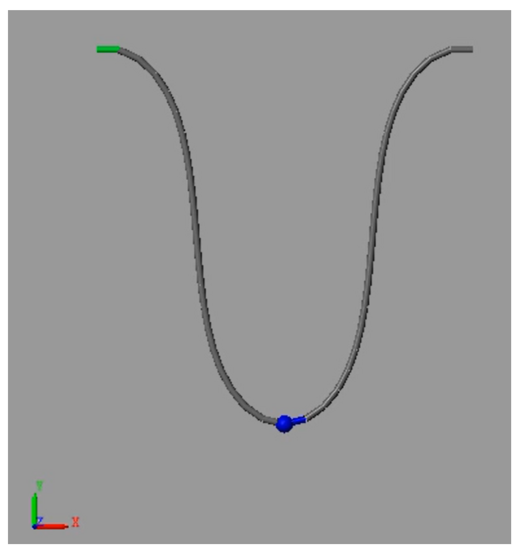
Figure 3 is a representative screenshot from the video that shows the dynamic behavior of the V-shape system returning to rest state. This validates the physical assumptions for the design of the proposed mechanical model. Moreover, it confirms that the V-shape system does not acquire a droplet shape, which is crucial for guaranteeing the monotony of the output signal provided by the flex sensor mounted at the ballast [
27]. This embedded instrumentation provides a suitable signal related to the compliance state that is appropriate for use as feedback for the winch command.
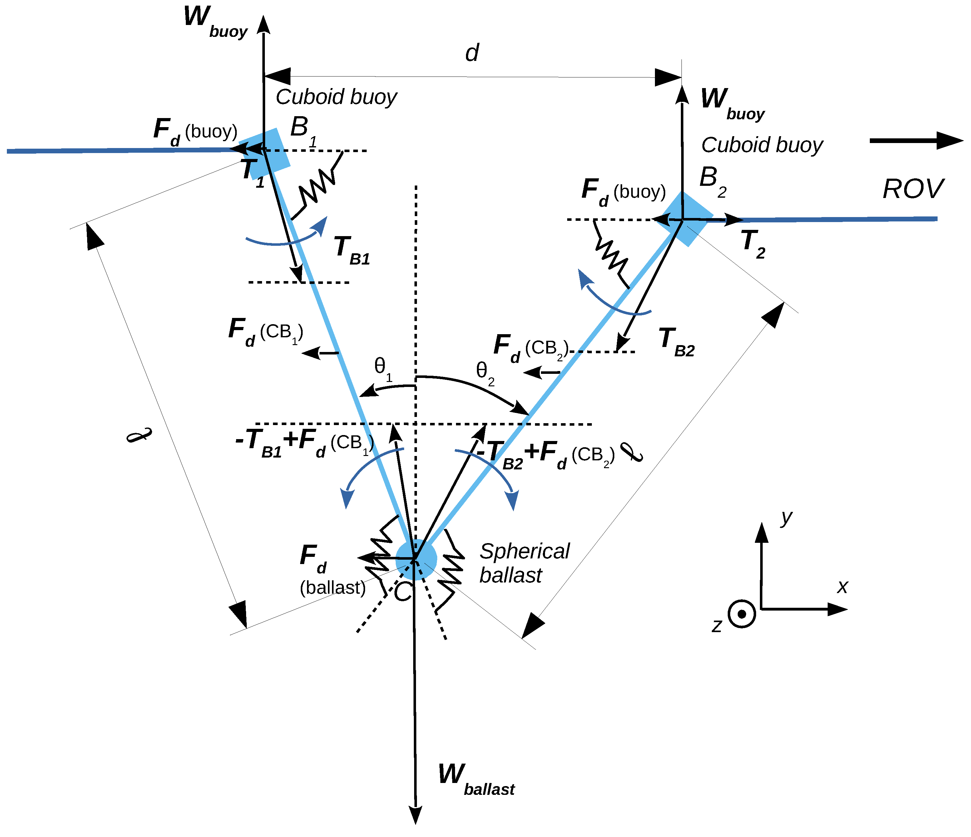
The V-shape system should not be excessive in size with respect to the robot’s dimensions. A distance of 1.2 m between the buoys was chosen for a 1 m range of distance compliance between buoys and a minimal distance of 0.2 m at rest, which yields ℓ = 0.6 m for each section and . The value of was set to approx. 36 .
3.2. Configuration for the Simulator
Simulations of the complete system, including the cable, buoy–ballast system, ROV (which is speed-controlled in open-loop), and cable feeder, were carried out using the Vortex
® simulator, version 2021a (2021.1.0.66). This software integrates the modeling of cables from a mass–spring model, taking into account their physical parameters for realistic rendering. The tether is a complex non-homogeneous object comprising several twisted strands and different coating layers. Some of its physical parameters are assumed to be constant and are directly provided by the manufacturers or easy to measure directly through experimental setups. Other parameters are more difficult to determine, requiring the use of abacuses.
Table 1 summarizes the parameters used for simulation. The simulated tether mimics the Fathom Slim tether. Breaking strength, radius, and linear density were obtained from datasheets. Bending stiffness, torsional stiffness, axial stiffness, damping, and drag coefficients were determined through experiments [
6].
The simulated ROV is adapted from the BlueROV2-Heavy from BlueRobotics™, which has four vertical thrusters and four thrusters for the horizontal movements arranged in vectorial mode.
3.3. Study of the Distance between Buoys
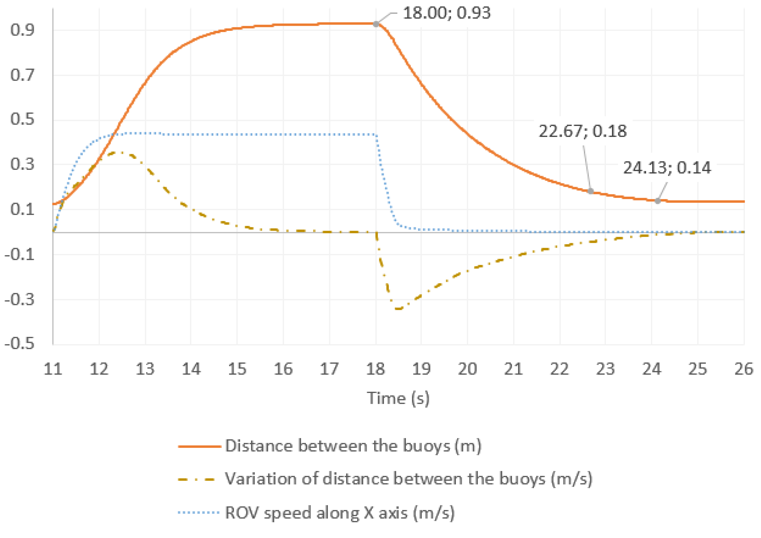
The distance between both buoys and its variation are observed while the ROV moves forward at a constant speed (
Figure 4). The coordinates of the centers of the buoys are used to calculate the distance and the variation. In this simulation, the ROV starts at a horizontal distance of 4 m from the remote station and a depth of 0.5 m. A length of 10 m of cable is unwound and then, at 11 s, the ROV starts to move 7 s forward at a controlled speed of 0.4 m/s. The desired speed is reached after 1.3 s. During the simulation, the difference between the length of the deployed cable and the distance of the ROV from the remote station is greater than 3 m. The time evolution of the distance between buoys shows that the system returns to its rest position in 5.5 s after the ROV stops. The 5% response time is 3.8 s. Thus, the system behaves like a damper. The impact of the 120 ms delay of the flex sensor, due to filtering post-processing, is negligible, and the acquisition/control frequency of 25 Hz is sufficient. Despite the damping effect, the variations in ROV speed immediately affect the distance between the buoys, which supports the interest in using this parameter to control the automatic distribution of the cable.
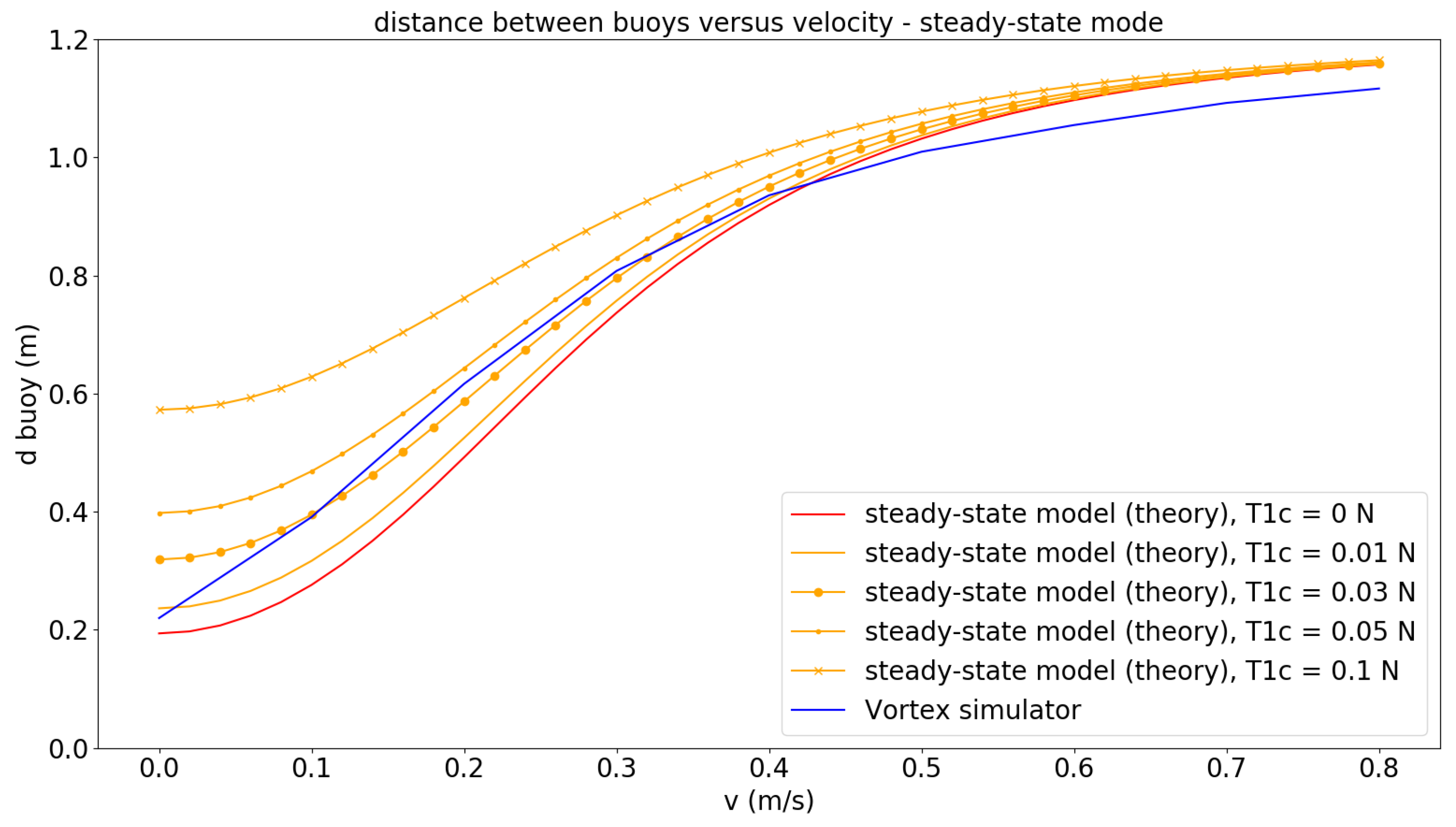
To observe the behavior of the damped system, the relationship between the distance between the buoys and the ROV forward speed at 0.5 m depth is shown in
Figure 5. The figure displays the curve obtained from simulation and the curves obtained from the theoretical model for values of
equal to 0 N, 0.01 N, 0.03 N, 0.05 N, and 0.1 N. The drag forces were considered quadratic. Despite some slight offset, the curve issued from the steady-state model with an order of magnitude of 0.03 N for
is close to the curve obtained in the simulation. The value of
depends on the design of the feeder built for the simulation. The inter-buoy distance is close to its maximum when the ROV reaches a speed of 0.8 m/s. This value represents the speed limit for optimal behavior of the system. The distance versus speed relationship can be used to define a target inter-buoy distance as a function of the ROV speed to help the system converge to the steady-state mode. this is not possible since labels are not compatible with tex symbols
3.4. Influence of Buoy–Ballast System on ROV Power
The power of the ROV is calculated using the manufacturer data of the T200 brushless motors that equip the BlueRov. The manufacturer datasheets provide the motor power as a function of the motor speed, and the thrust as a function of the motor speed. The motors’ speeds are controlled to achieve the desired vehicle speed. The total power is then calculated by summing the motor powers.
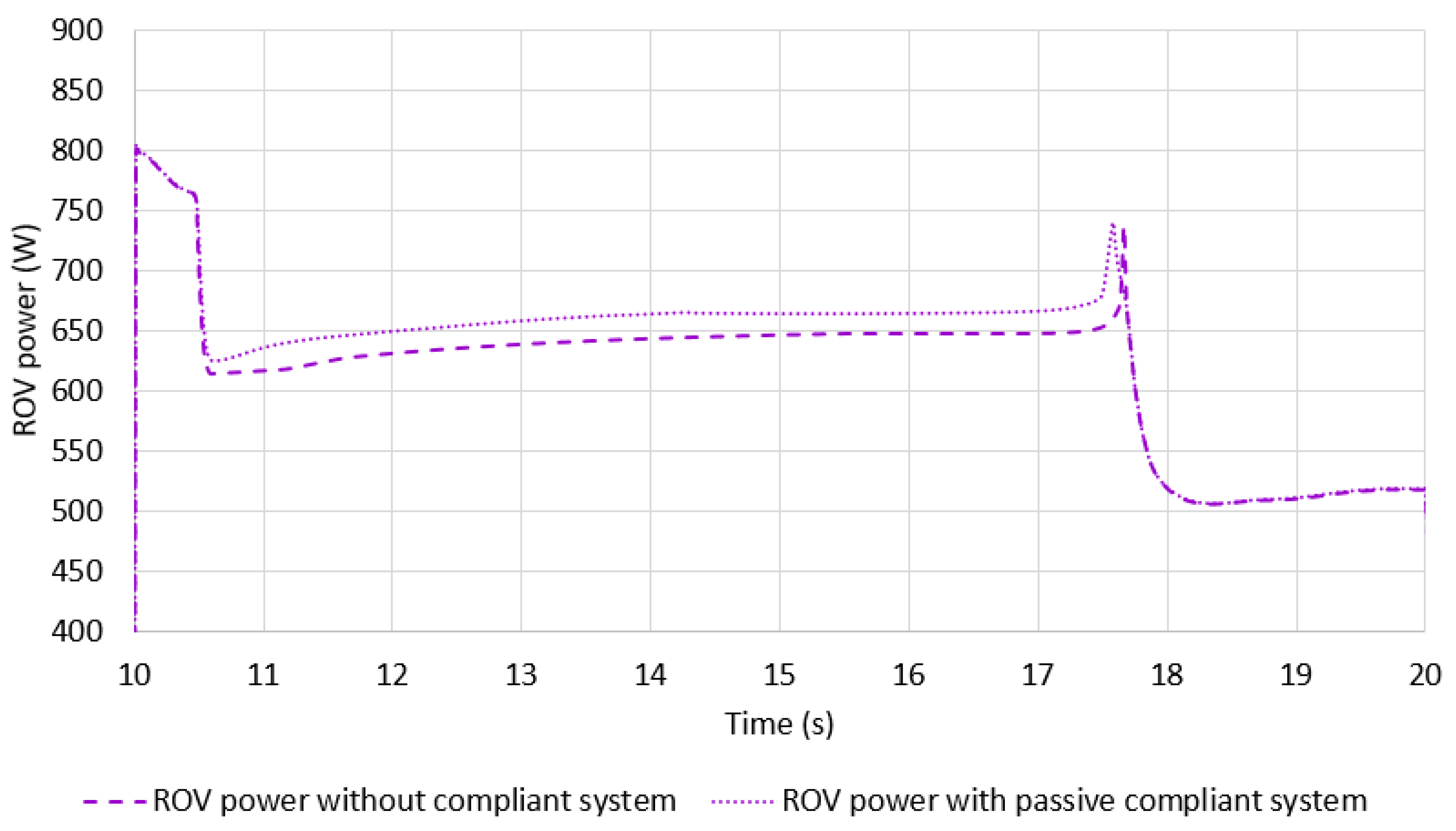
The speed of the ROV is not affected by the presence of the compliant system since the simulated ROV is velocity-controlled. However, the total power of the ROV thrusters observed in simulation, represented in
Figure 6, is
higher globally with the compliant system. This is due to the drag forces on the buoy–ballast system that the cable transmits to the ROV. The passive compliant system introduces slightly more tension in the cable throughout the movement of the ROV compared with a free cable with sufficient length. However, this increase in tension is not significant, and the compliant system on the cable prevents the cable from pulling strongly on the ROV.
3.5. Generation of ROV Trajectories for Further Analysis
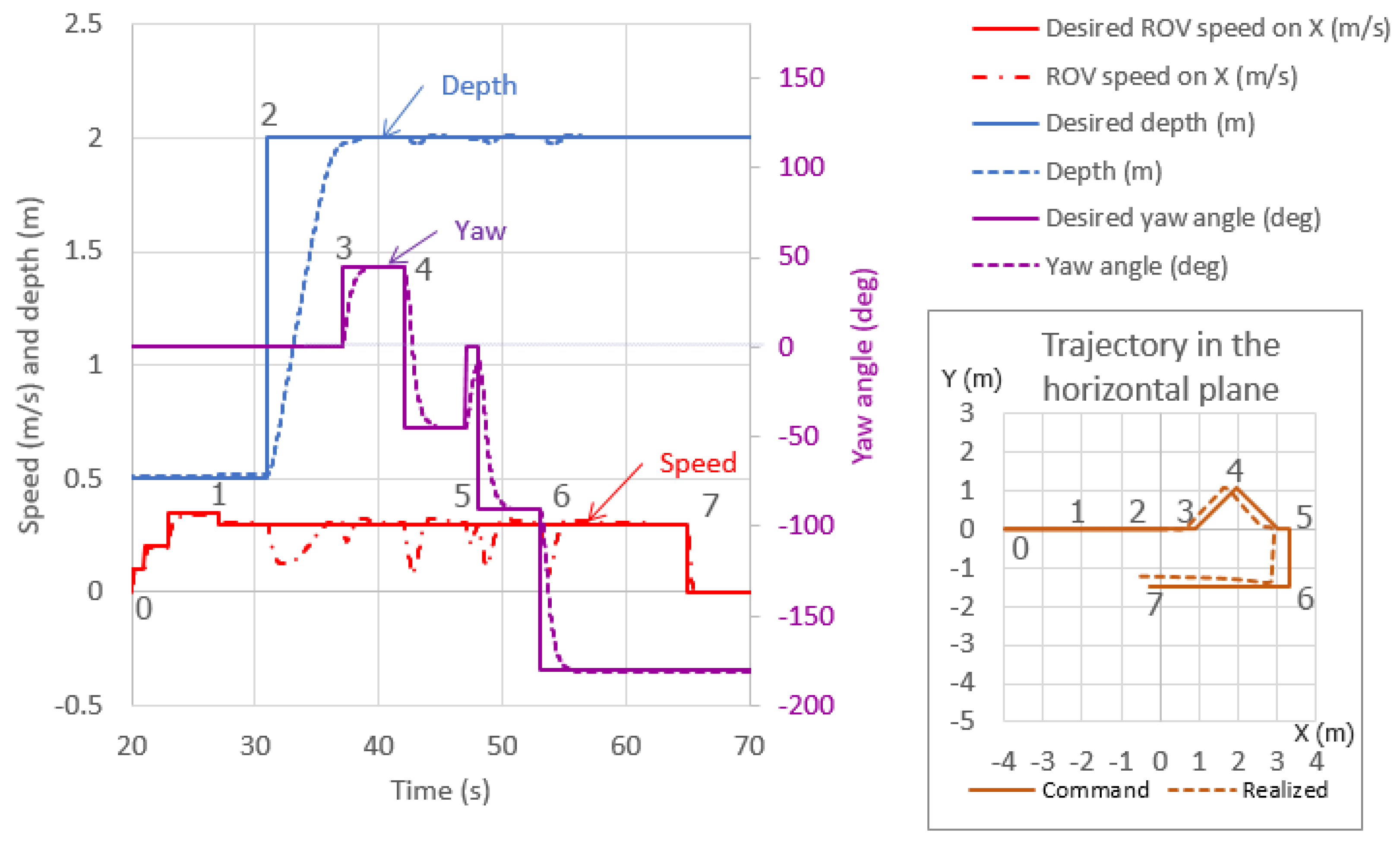
Generation of trajectories. Trajectories are defined as a sequence of depth, orientation, and speed commands of the ROV. The ROV is speed-controlled with a PID control loop and with a proportional control loop in heave, yaw, roll, and pitch.
Figure 7 presents the curves for the velocity, depth, and angle commands as well as the values measured during the simulation for an untethered ROV. Keyframes are indicated on this trajectory to provide reference points. This trajectory starts with forward movement of the ROV along its longitudinal axis at different successive speeds between points 0 and 1 (0.1 m/s, 0.2 m/s, and then 0.3 m/s) in parallel with a depth control of 0.5 m. Then, a command for a forward speed of 0.3 m/s is sent again (point 1), followed by a depth command at 2 m (point 2). Then, while moving forward at a constant speed, the ROV receives successive yaw commands:
to the left (point 3),
to the right (point 4),
,
to the right (point 5), and
(point 6). Finally, the forward speed command is set to zero, while the depth command is kept to 2 m (point 7). The trajectory projected in the horizontal plane, deduced from the longitudinal speed and the orientation of the ROV, is also presented at the bottom right. The difference between the set point and the actual displacements of the ROV is due to hydrodynamic phenomena, which slow down the ROV in water. Moreover, when there are changes of set point in depth and yaw, a significant acceleration is required, resulting in overloading of the thrusters and affecting the speed along the
x-axis (
Figure 7).
Control schemes. The behavior of the system is compared for five different modes listed below.
Cable not controlled and without compliant system: the cable length is fixed to 15 m along the simulation.
Cable with passive compliant system (not controlled): the cable length is fixed to 15 m along the simulation.
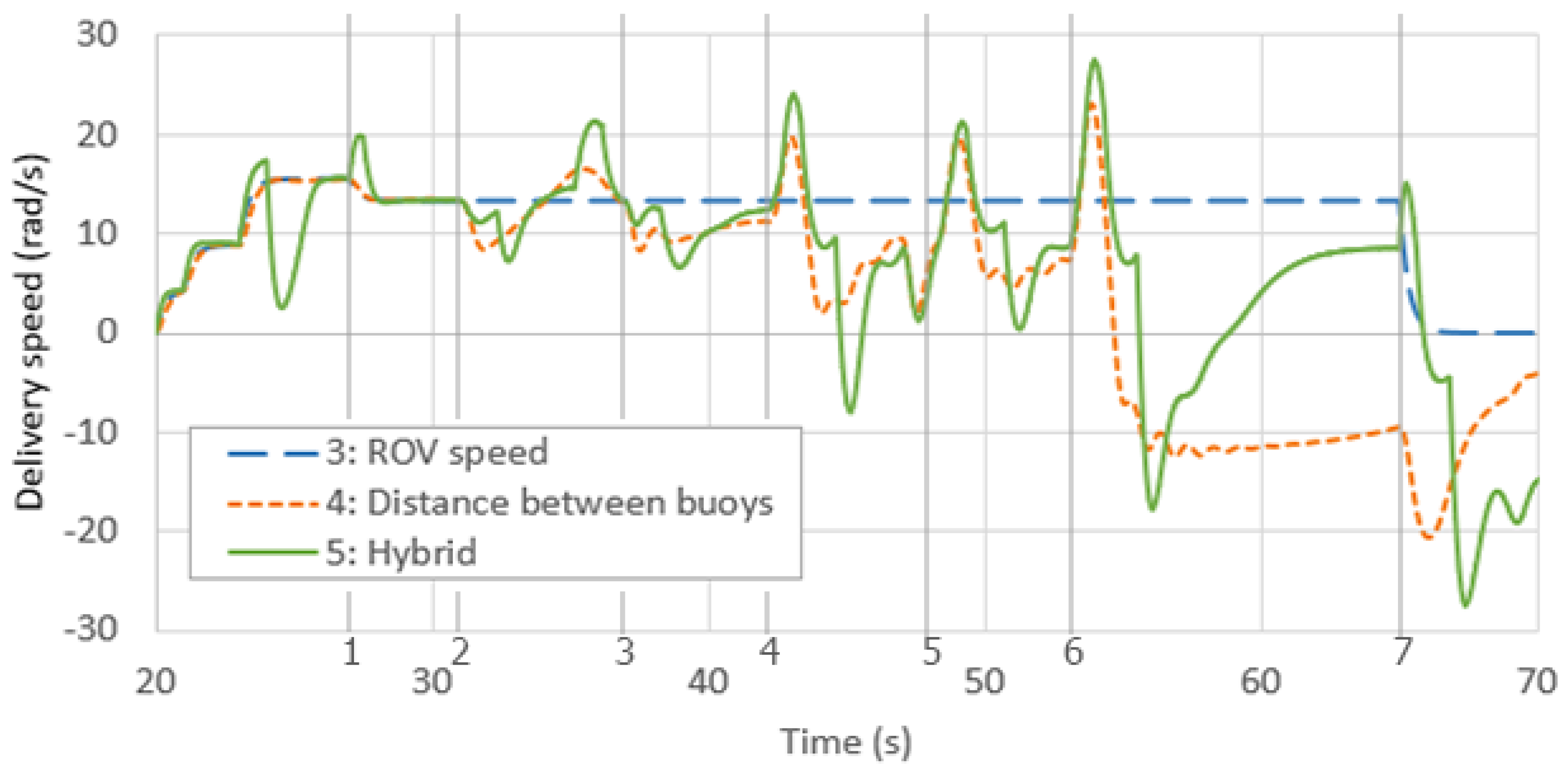
Cable controlled with ROV speed command as input: the delivery speed of the cable is set to the ROV speed.
Cable controlled with distance between the buoys: a closed-loop PD controller maintains a target distance of 0.8 m between the buoys.
Hybrid control of the cable based on ROV speed and distance between buoys, which combines buoy distance PD controller and P controller using an ROV speed command. Furthermore, the target distance between the buoys is set to vary according to the ROV speed. The proportional part of the PD controller on the buoys’ distance works only if the distance is at least 5 cm longer than the target (taut cable) or if it is less than the target for more than 1 s (slack cable).
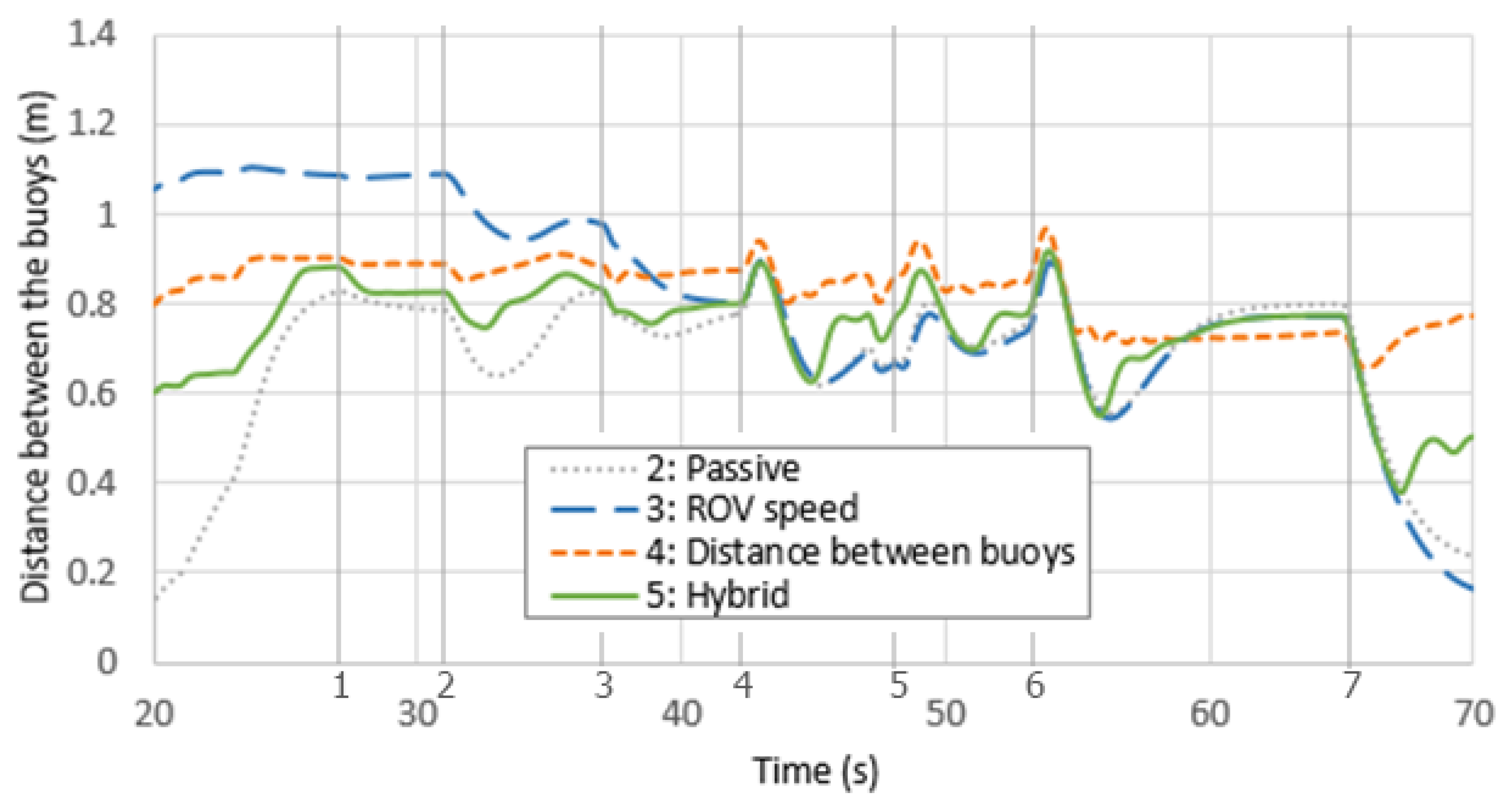
Distance between buoys.
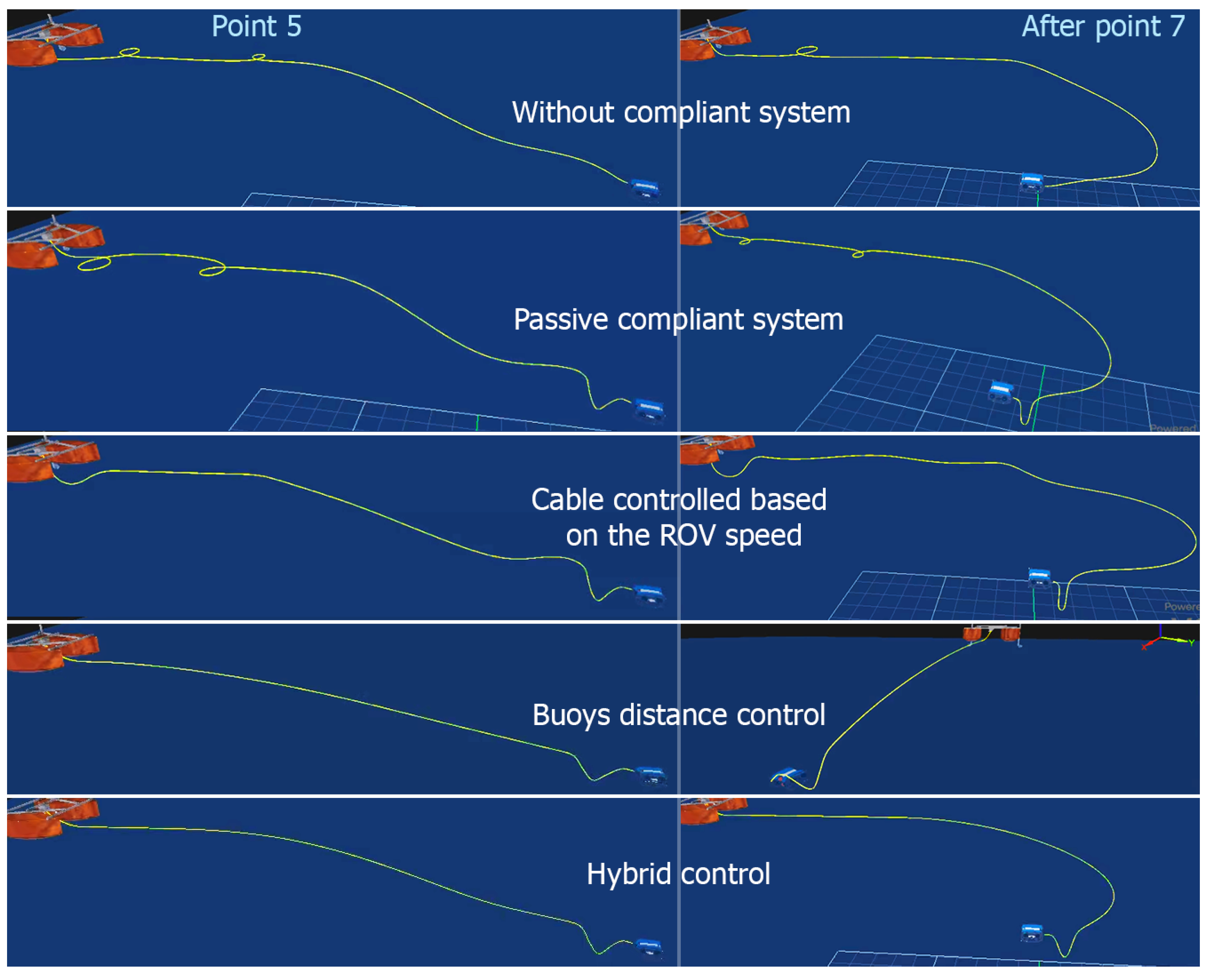
Figure 8 depicts the evolution of the distance between buoys for passive configuration and the three control modes.
Unsurprisingly, the best control is obtained with the buoy distance-based control, which keeps the distance between buoys around 0.8 m, despite oscillations that appear when the ROV is turning, from keyframe 3 to shortly after keyframe 6. The hybrid controller allows the distance to be kept within reasonable values, between 0.4 m and 0.9 m. The distance between the buoys reaches more extreme limits (0.16 m and 1.1 m) when the cable is not controlled or ROV speed-controlled.
Cable delivery speed.
Figure 9 shows the delivery speed for the three control modes.
When the ROV moves forward at low speed (before keyframe 1), the feeder’s speed is almost the same for the three control modes. As only the linear speed is considered for the ROV speed-based control, the cable delivery speed remains constant between keyframes 1 and 7, not taking into account the orientation of the ROV. Oscillations are more pronounced for the hybrid controller than for the buoy distance-based controller, resulting in a smoother cable delivery speed.
Overall cable shape. The overall shape of the cable is depicted in
Figure 10 for all cable control configurations at two different keyframes of the trajectory, namely keyframe 5, when the ROV finishes its forward motion, and after keyframe 7, when the ROV returns close to the feeder. With the hybrid control, the cable behaves correctly, except for when a slight excess of cable forms a lobe as the ROV moves toward the feeder. The length of free cable is too long with the ROV speed controller. In contrast, the length of free cable is tightly adjusted when using the buoy distance-based controller. When the cable is not controlled, loops appear on the water surface before the ROV starts to move away, as the cable length is far too long. These loops remain throughout the trajectory, generating a significant risk of snagging or entanglement of the cable.
Conclusions from controller analysis.
Of the three controllers evaluated in the simulation, the ROV speed-based controller is not sufficiently responsive and generates a static error on the buoys’ distance that is never corrected. It is therefore not robust to external disturbances.
The control mode based on the distance between buoys is rather smooth, robust, and reactive.
The hybrid control is quite reactive but presents some more pronounced oscillations while remaining rather stable. Hybrid control could possibly be improved by replacing the ROV command speed with the actual ROV speed, which would require the use of more sensors on the ROV, such as a Doppler velocity log (DVL).
4. Description of Setup, Control Mode, and ROV Trajectories for Real Experiments
The simulations described in the previous section allowed validation of the behavior of the V-shape system by comparing the different modes of cable control. This section describes the preparation for real experiments that took place in water tanks. This preparation includes the setup, control scheme, and two kinds of trajectories that were used to check the system behavior in real conditions. To ensure the ground truth of the movements of the cable, compliant buoy–ballast system, and ROV, an underwater motion capture system was implemented.
4.1. Setup
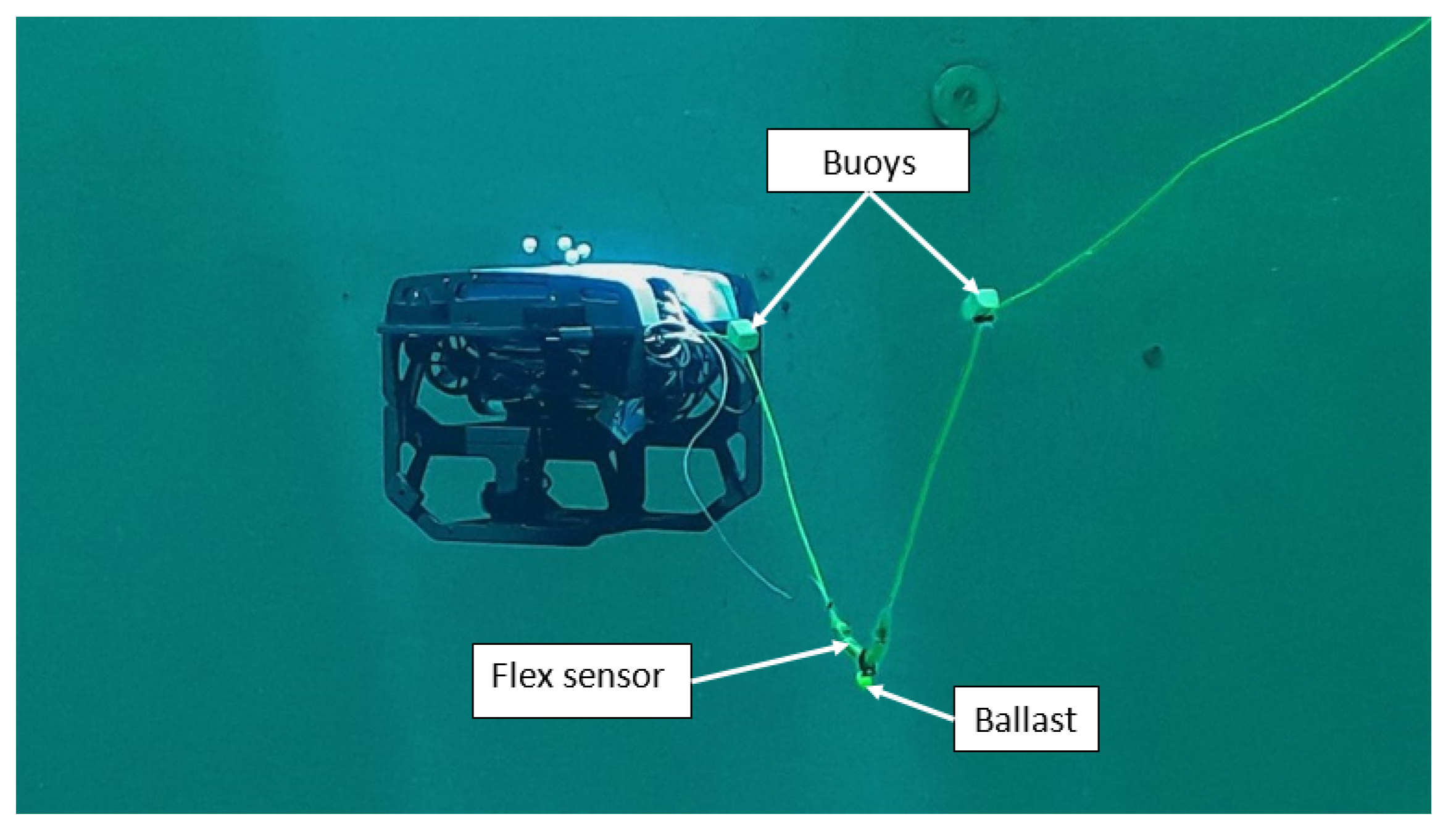
The cable feeder was fixed on the border of a 16 × 8 m water tank and connected to the ROV through a 25 m long 4 mm diameter tether, namely the Fathom Slim, equipped with the buoy–ballast system, of which a technological description can be found in [
27]. The ROV used was a BlueROV2-Heavy, as in the simulation.
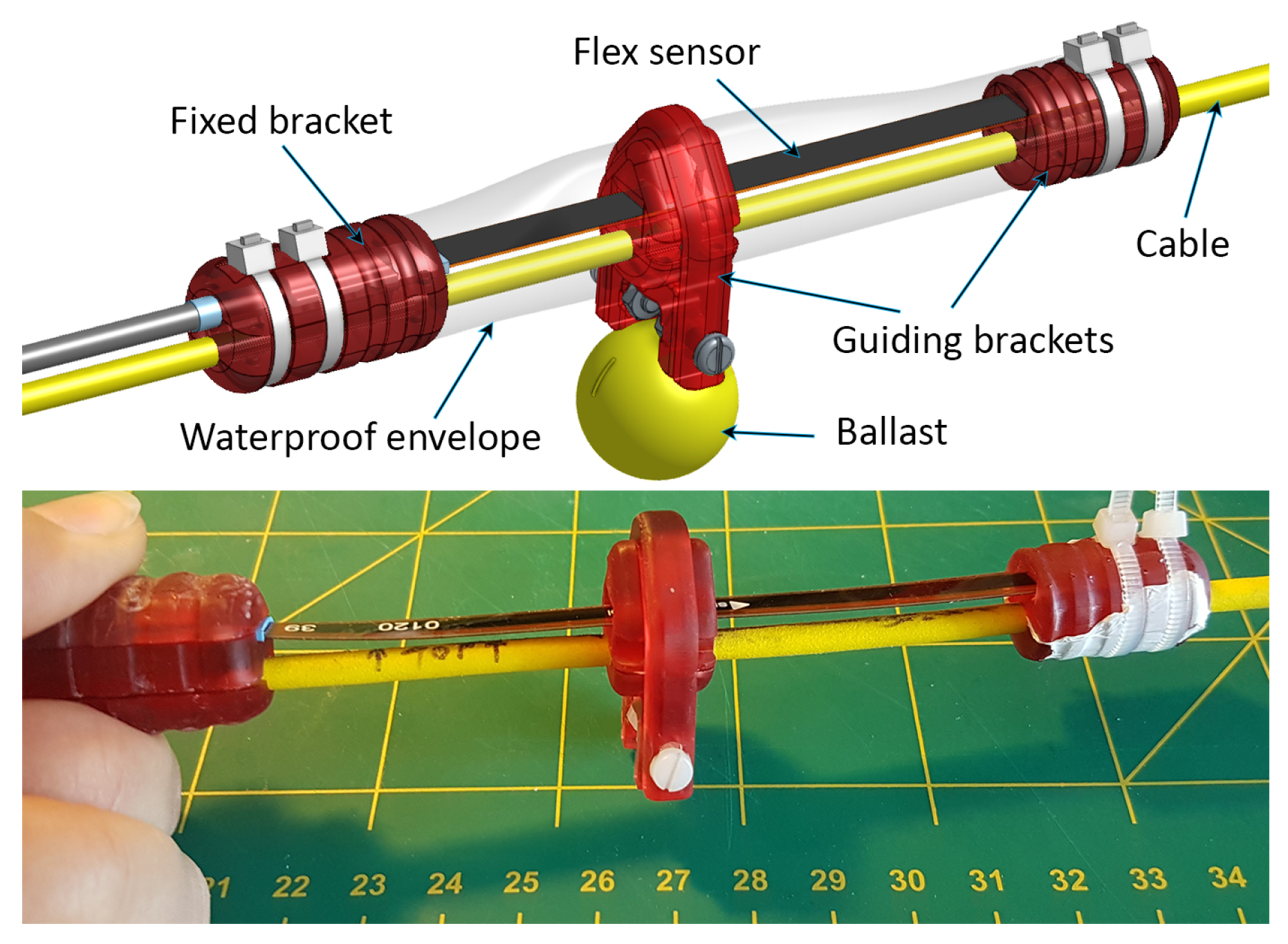
A flex sensor was mounted on the cable at the ballast location using a fixed bracket and guides along the cable (
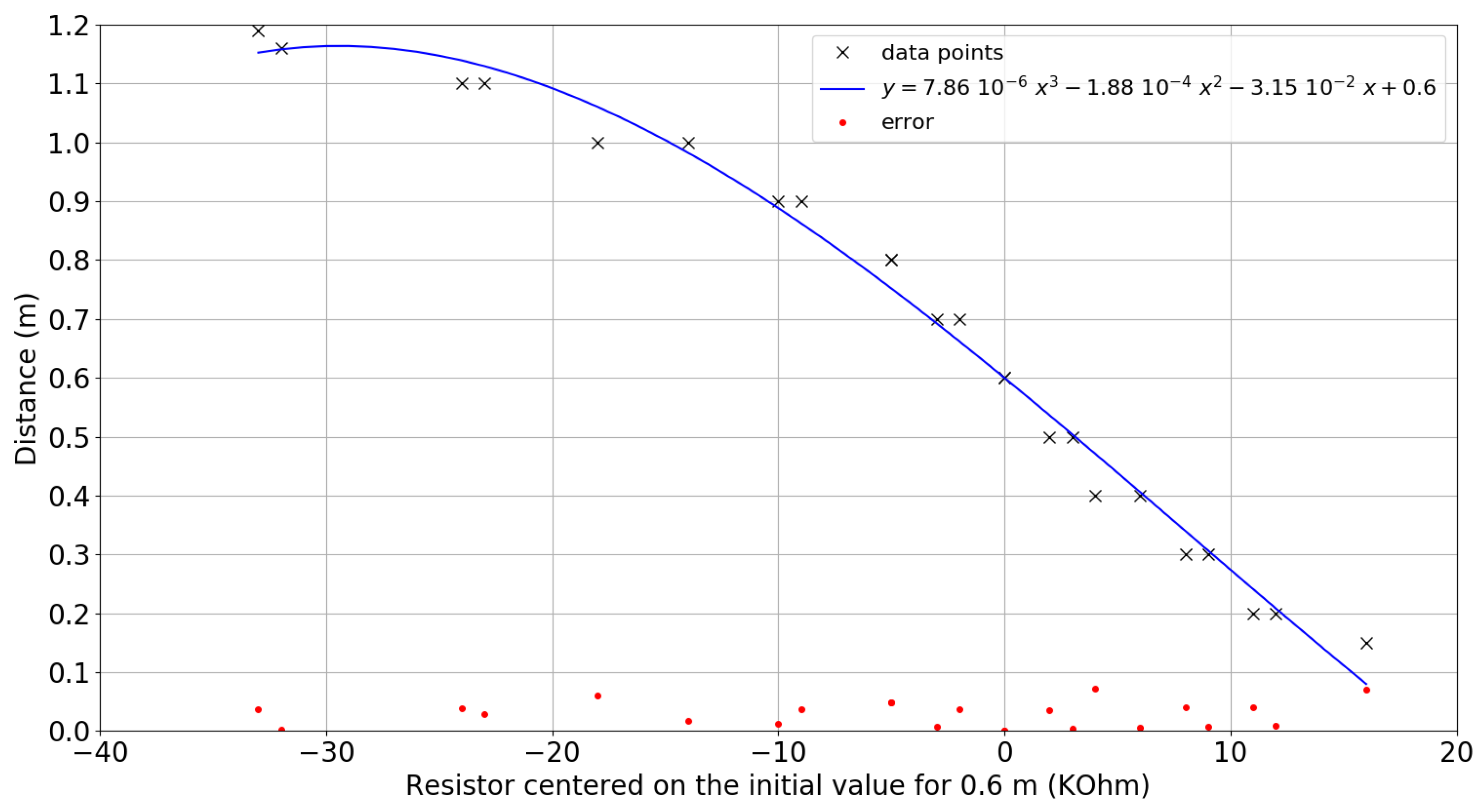
Figure 11). The sensor has negligible bending stiffness. It was wrapped in a thin plastic envelope for waterproofing. The sensor resistance varies when the cable is bent. This varying resistance is transformed into a voltage signal through a voltage divider, then filtered, centered, and trimmed. The variation in the resulting signal is used to fit the corresponding distance between the buoys through a third-order polynomial (
Figure 12).
Table 2 summarizes the characteristics of the buoy–ballast system to which the Fathom Slim tether is equipped, taking into account the previously described modeling analysis.
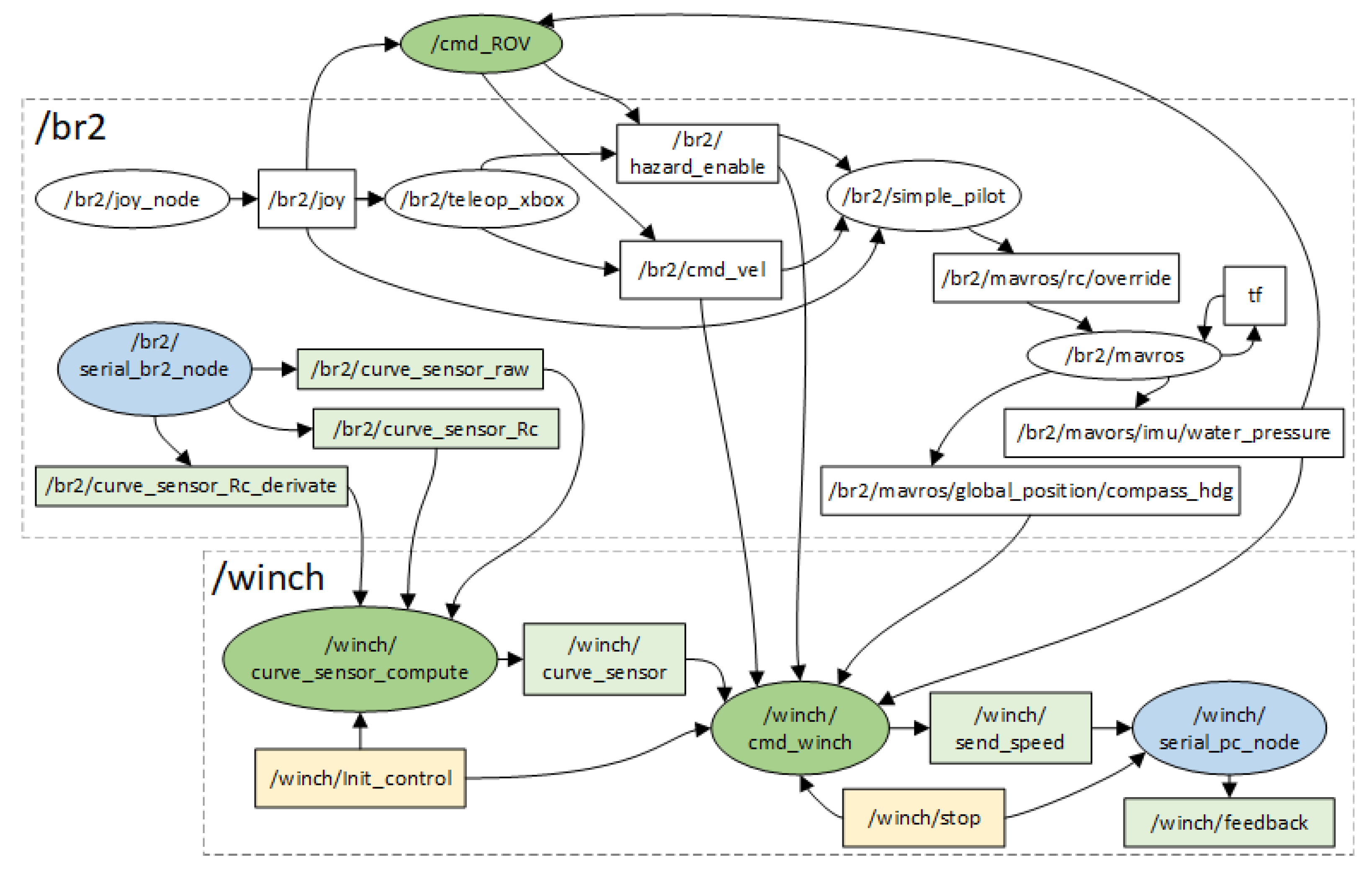
The controller board inside the robot was run on a Linux/ROS-1 system with the
mavros library to interface the high level control with the autopilot
ArduSub. The BlueROV2 was controlled remotely via a gamepad connected to the control computer. The remote control computer contains the embedded ROS
master. It was connected to the feeder for the transmitting of control commands while taking into consideration the data received from the flex sensor through the ROS system embedded in the robot. The diagram in
Figure 13 shows the architecture of the ROS
nodes for controlling the global system during the experiments.
The robot and the cable were tracked by a camera motion-tracking system, namely Qualisys, with five underwater optical cameras Miqus M5u at 180 frames per second. The cameras use blue LEDs, whose light is reflected by markers placed on the ROV and the cable. Data are recorded from the QTM software, version 2020.3 build 6020, which is controlled from a dedicated computer during the experiments. This software computes the current 3D position of each marker provided they are detected by several cameras. Across the experiments, the position residuals of the markers were about 1.3 mm for the ROV, with a minimum of 0.9 mm and a maximum of 10 mm.
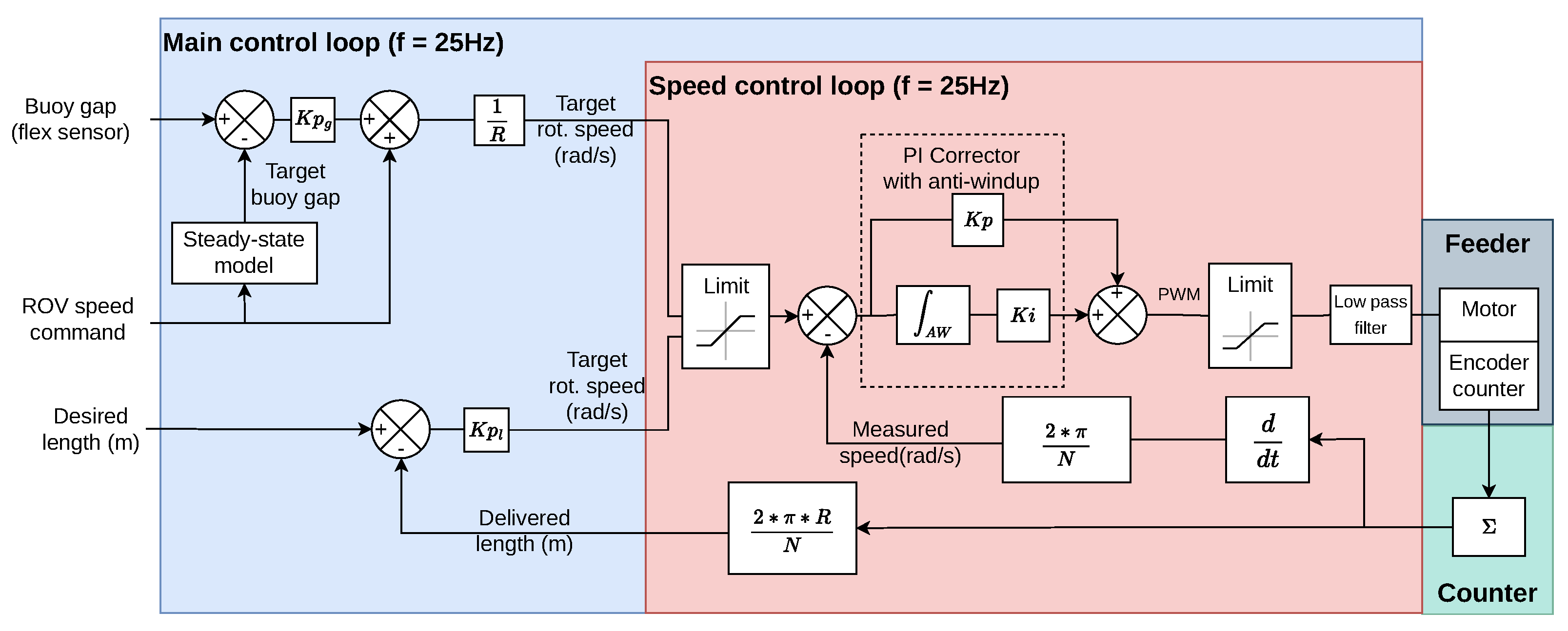
4.2. Control Scheme
Figure 14 is the control block diagram of the feeder, which can be controlled using the measured distance between buoys, namely buoy gap on the figure, or using a desired cable length. The control for the feeder consists of a main control loop with proportional controllers, which includes a speed control loop with a proportional–integral controller and anti-windup system. Flex sensor processing, presented in
Section 4.1, is used to estimate the inter-buoy distance, which is sent to the feeder by the ROV.
In normal mode, namely buoy gap control mode, the feeder speed is controlled as the ROV moves to regulate the gap between both buoys. The target buoy gap is defined from the actual ROV speed using the steady-state model that gives the variations in the buoy gap as a function of the ROV speed (see
Section 2.3 and
Figure 5). The target buoy gap is then compared to the current gap measured by the flex sensor to update the rotation speed of the feeder.
In length control mode, the cable length can be directly controlled by setting a desired length. The feeder can actually be operated to release the cable when necessary; e.g., when the V-system is stretched, 2 m of cable is uncoiled after a 10 s period until the V-system is released.
Buoy gap control and length control modes are separately activated as required. Cable length is computed in the speed control loop such that it is accessible even when length control is disabled. The target rotation speed is first bounded to avoid exceeding the motor limits. Embedded in the speed control loop is a proportional–integral corrector, which is applied to the error between the bounded target speed and the measured speed. This corrector has an anti-windup system that limits the sum of past errors to stabilize the system. It outputs a raw PWM signal, which is then bounded and smoothed by a low-pass filter before being transmitted to the motor control board.
4.3. Trajectories
The experimental results of cable control validation were obtained during a series of tests carried out in the pool of the CIRS (Underwater Robotics Research Center) in Girona in the context of a TNA (TransNational Access) European project.
Two kinds of ROV trajectories were defined to represent two configurations where cable control must be useful to reduce risks of cable snagging or entanglements as below.
A linear trajectory where the ROV goes forwards and then backwards First, a forward thrust command of is sent for 15 s (between keyframes 1 and 2). Then, a zero command is sent for 5 s (between points 2 and 3). Finally, a backward thrust command of is sent for 10 s (between points 3 and 4).
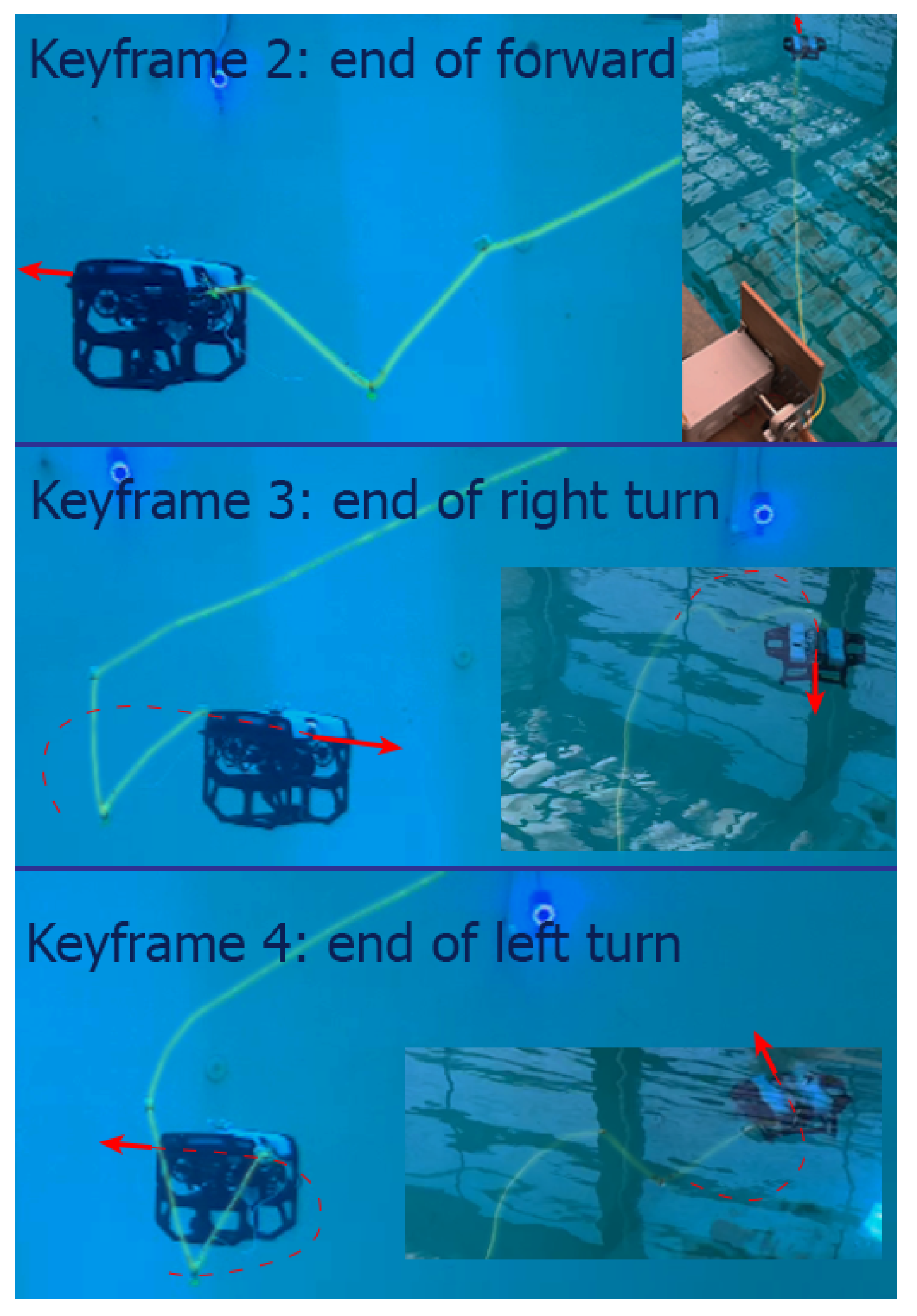
A curvilinear S-shape trajectory comprising the following steps:
- -
a forward thrust of 40% for 15 s (between points 1 and 2);
- -
a right turn composed of a yaw thrust of combined with a forward thrust of for 6.5 s to turn right (between points 2 and 3);
- -
a left turn with the same thrust command values as the left turn, for 6 s (between points 3 and 4);
- -
a forward thrust of for 4 s (between points 4 and 5).
All these trajectories were associated with 1.5 m depth control. The ROV was open-loop-controlled to follow these trajectories by driving the corresponding thrusters.
For each trajectory, three kinds of cable management were tested:
Passive slack cable, where cable of sufficient length was deployed in the water from the beginning.
Passive taut cable, where the cable is stretched between the feeder and the ROV when the ROV moves away from the feeder, which means that the buoy–ballast system is also completely stretched and has no real influence on the ROV. The feeder is not powered. When the ROV comes closer to the feeder, the cable is no longer taut, and the buoy gap tends to be reduced to a minimum.
Cable control, using buoy gap control mode. A and forward thrust is associated with a buoy gap of about 0.7 mn and 0.8 m, respectively, according to the steady-state model.
5. Results And Discussion
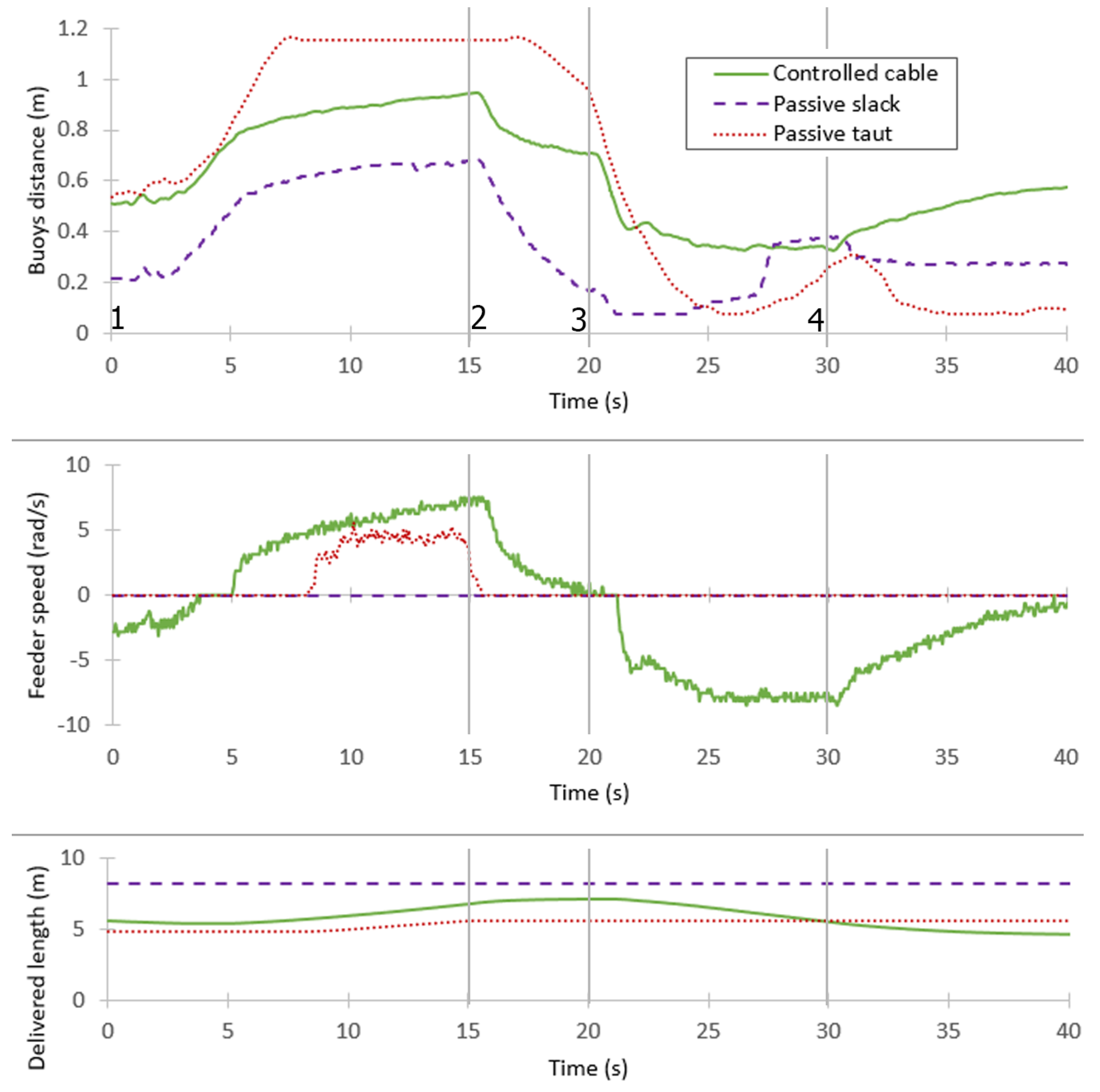
5.1. Linear Trajectory
Figure 15 illustrates the cable management results for the linear trajectory including buoy distance control mode, passive slack mode, and passive taut mode. The feeder appears to be quite reactive and smooth in winding/unwinding the cable depending on ROV motion and the distance between buoys. The buoy–ballast system exhibits highly dynamic transient behavior between points 2 and 4 due to the changes in velocity. When moving backward, the feeder also takes more time for buoy gap convergence back to the target distance (0.7 m).
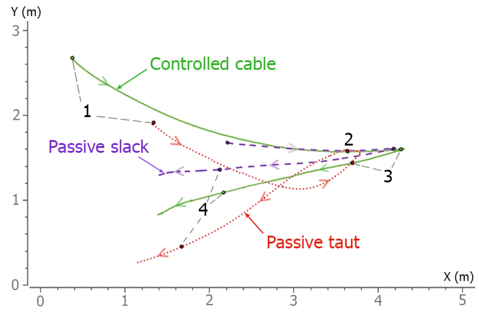
Figure 16 presents the paths followed by the ROV projected onto the horizontal plane as measured by the
Qualisys system for the three cable modes.
If there were no external disturbances at all, the path would be rectilinear. The ROV shifts slightly to the left when the cable is slack. This deviation is slightly larger in the control mode and is observed during both its forward and backward motion. The deviation is significantly greater in passive taut mode. Furthermore, the distance covered by the ROV is shorter with the taut cable.
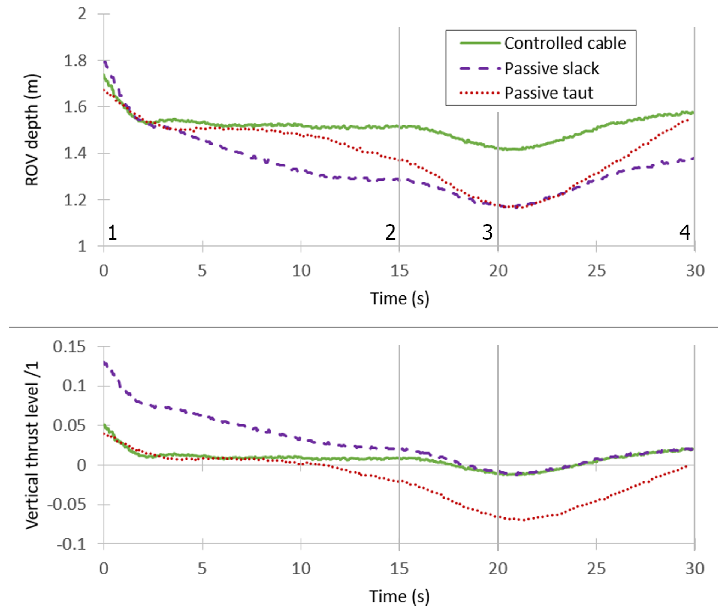
Figure 17 shows the evolution of depth control of the ROV for the three modes. Only the control mode is efficient in helping to regulate the ROV depth. In addition, the vertical thrusters’ work significantly increases more when the cable is not controlled than when it is controlled.
5.2. Curvilinear Trajectory
Figure 18 shows the snapshots at keyframes 1, 3, and 4 in cable control mode.
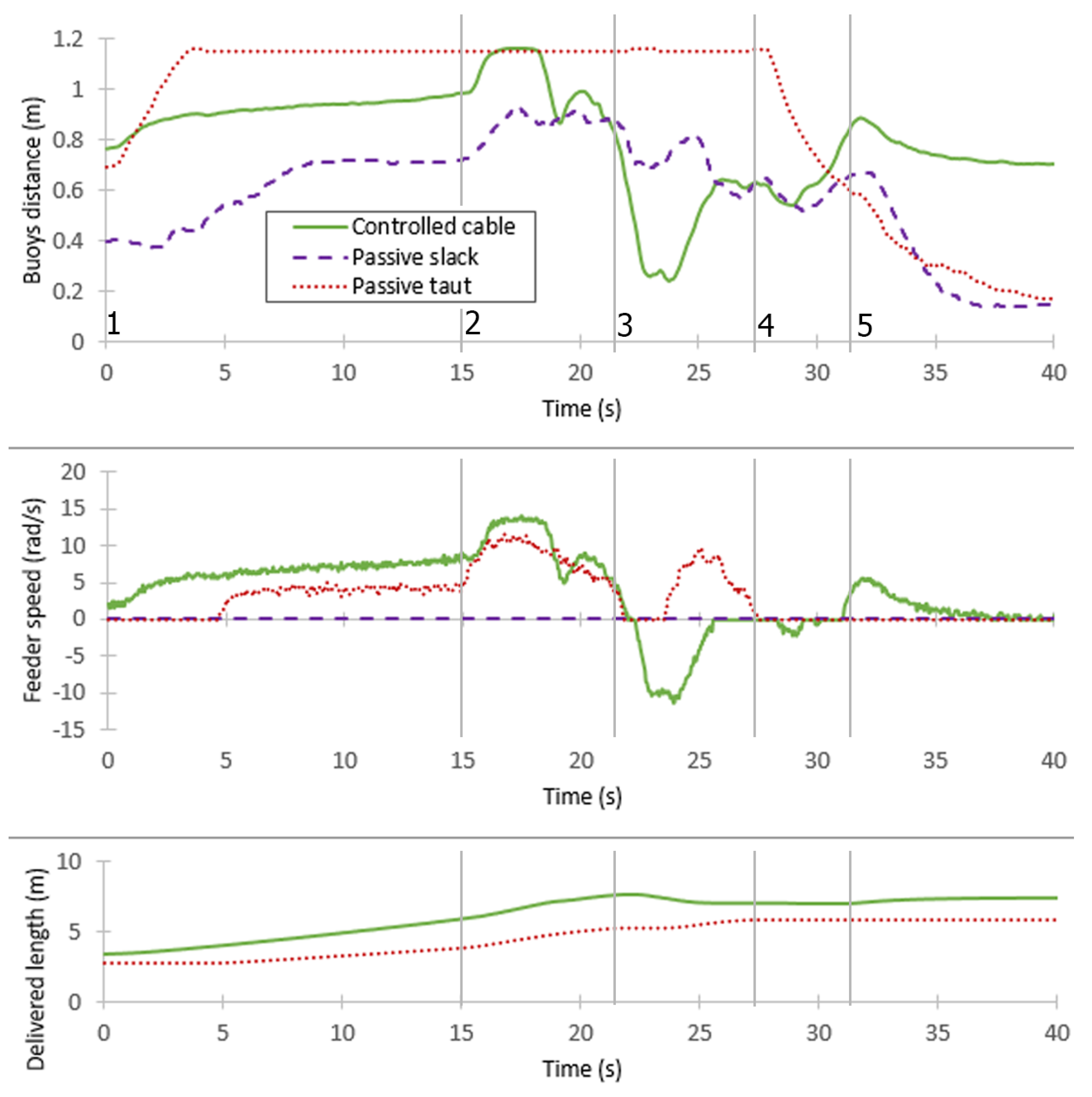
Figure 19 presents the results in terms of buoy gap, feeder speed, and delivered cable length.
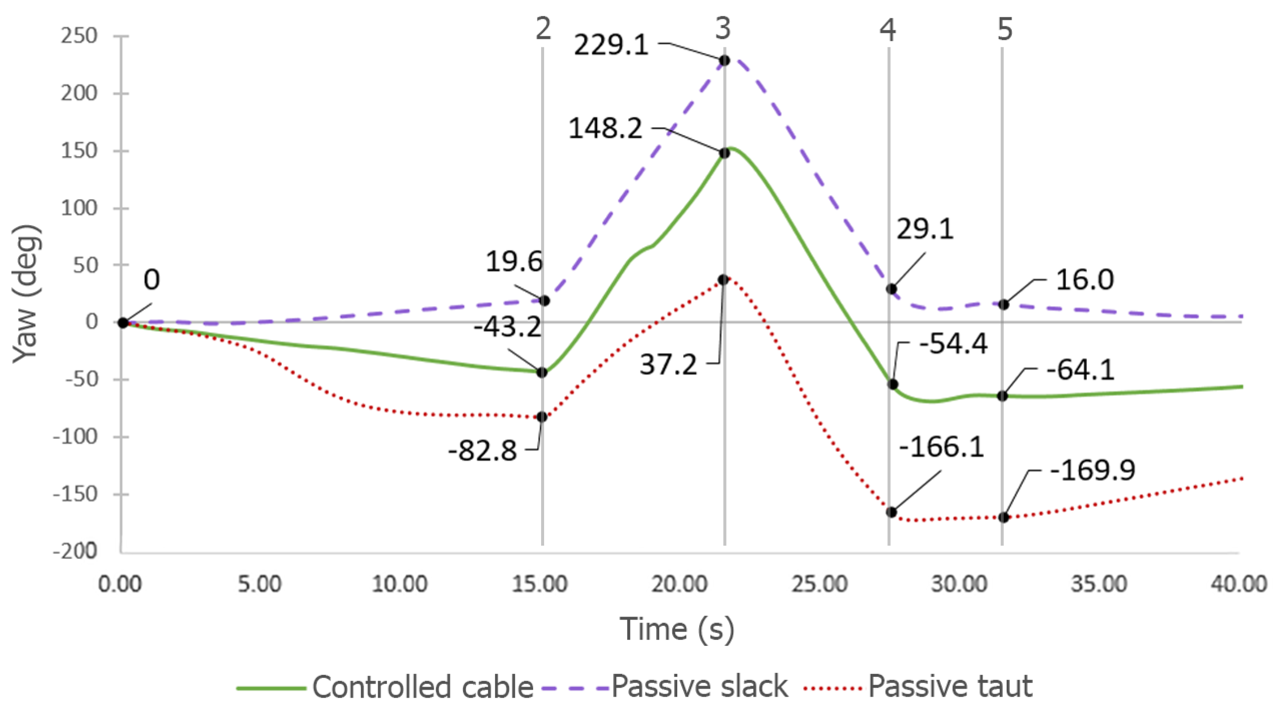
Figure 20 presents the yaw angle.
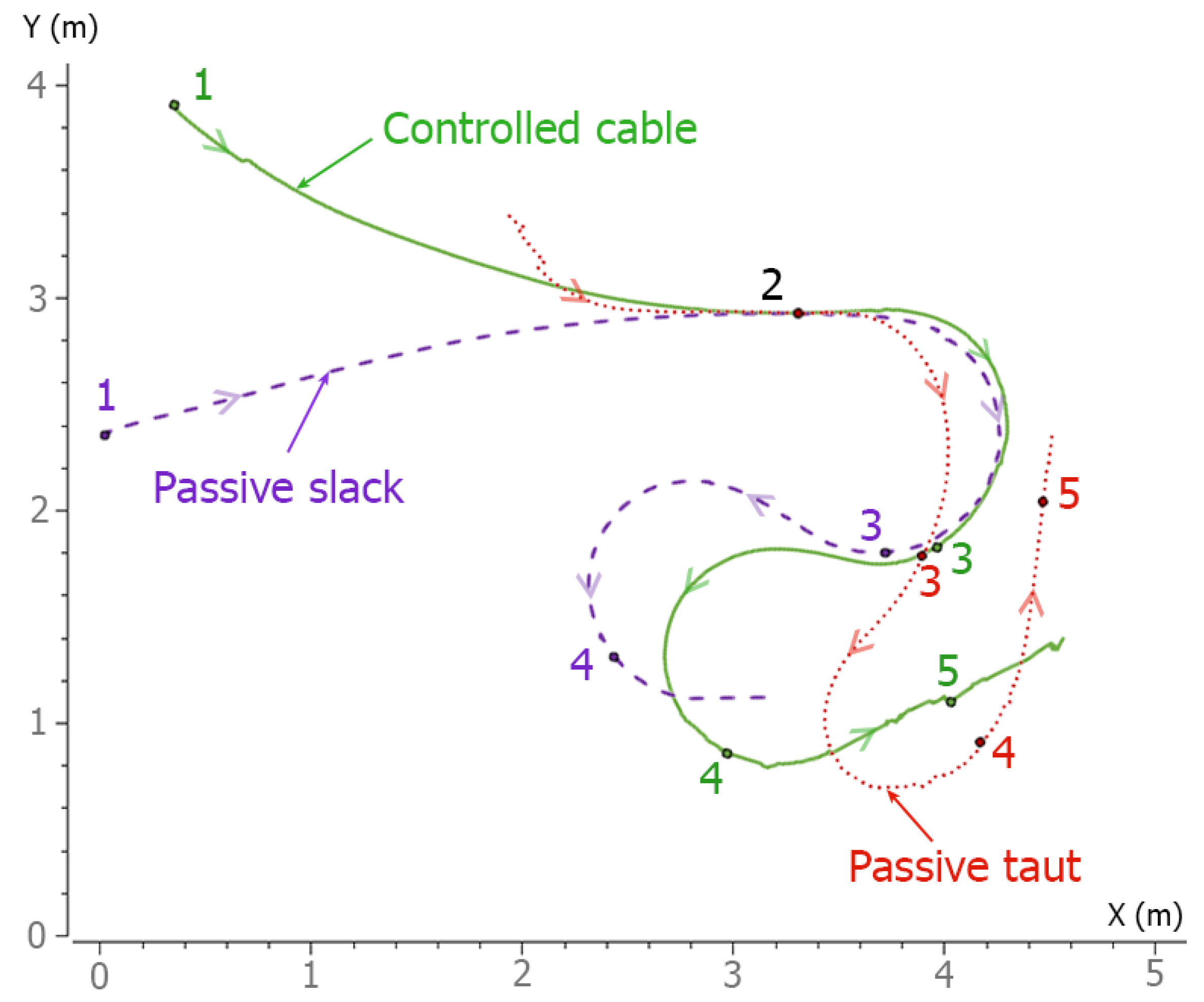
Figure 21 shows the executed trajectories in the cases of passive slack cable, passive taut cable, and control mode.
In control mode, the compliant system keeps its V-shape and a buoy gap average close to the target distance (0.8 m), except for during turns, where the behavior is highly dynamic because of the increased forward speed and the opposing directions of the successive turns, which causes the buoy gap to reach its bounds, namely 0.2 m and 1.2 m, during a short period of time. The buoy gap resulting from passive taut and passive slack modes demonstrates the added value of automatic cable length management in maintaining an average buoy gap, which allows the cable shape between the station and the buoy–ballast system to be controlled.
For a flawless system without any disturbance, the yaw angle (
Figure 20) must be constant during the ROV straight line commands (before point 2 and after point 5). It must also be linear during rotating commands (between points 2 and 3, then 3 and 4). There is a slight deviation of about 20 deg to the right during the first straight line (2.6 m) command of the ROV for the passive slack cable. This deviation is oriented to the left and its absolute value is doubled with the controlled cable and doubled again with the passive taut cable. In fact, the cable is fixed on the left side of the back of the ROV, which induces a slight deviation to the left for the controlled cable, both in a straight line and during a right rotation. This deviation is much larger for the passive taut cable. The left rotation of the ROV appears to be less affected in the control and passive taut modes.
The impact of these deviations is observed in
Figure 21, in which the ROV paths in top view are shown for the three modes.
The distances traveled are quite similar for the controlled cable and the passive slack cable, whereas the turns are slightly different. The path of the ROV with the passive taut cable is completely distorted. The first rotation to the right (between points 2 and 3) is tightly confined, and the rotation to the left (between points 3 and 4) is quite irregular (much wider curvature in the middle than at the beginning and the end).
The experiments also showed there is effective control of the cable using the compliant buoy–ballast system, which keeps the cable in a semi-stretched configuration, and the delivered length is appropriately managed, preventing the creation of cable loops that can occur in passive slack mode and reducing the risks of snagging and tangles, considering that turns in passive taut mode can cause the cable to become entangled with the robot. The control mode generates slight tension in the cable, which is transmitted to the ROV and results in a minor deviation in the trajectory of the system, which can be avoided by fixing the cable closer to the ROV’s center of gravity. In addition, the passive compliance system appears to improve the stability of the depth control of the ROV.


