UVI Image Segmentation of Auroral Oval: Dual Level Set and Convolutional Neural Network Based Approach

Abstract

The auroral ovals around the Earth’s magnetic poles are produced by the collisions between energetic particles precipitating from solar wind and atoms or molecules in the upper atmosphere. The morphology of auroral oval acts as an important mirror reflecting the solar wind-magnetosphere-ionosphere coupling process and its intrinsic mechanism. However, the classical level set based segmentation methods often fail to extract an accurate auroral oval from the ultraviolet imager (UVI) image with intensity inhomogeneity. The existing methods designed specifically for auroral oval extraction are extremely sensitive to the contour initializations. In this paper, a novel deep feature-based adaptive level set model (DFALS) is proposed to tackle these issues. First, we extract the deep feature from the UVI image with the newly designed convolutional neural network (CNN). Second, with the deep feature, the global energy term and the adaptive time-step are constructed and incorporated into the local information based dual level set auroral oval segmentation method (LIDLSM). Third, we extract the contour of the auroral oval through the minimization of the proposed energy functional. The experiments on the UVI image data set validate the strong robustness of DFALS to different contour initializations. In addition, with the help of deep feature-based global energy term, the proposed method also obtains higher segmentation accuracy in comparison with the state-of-the-art level set based methods.

1. Introduction

The aurora is a natural light phenomenon mostly observed around magnetic polar regions in both hemispheres. The energetic particles precipitating from solar wind interact with geomagnetic field and accelerate along magnetic field lines towards Earth [1]. These particles collide with neutral constituents in the upper atmosphere, which generates the most impressive wonder of Auroral Borealis and Aurora Australis [2]. More importantly, the structure of aurora is a mirror which reflects the physical process in the magnetosphere and assists the scientists to research the intrinsic mechanism in the solar wind-magnetosphere-ionosphere coupling process [3].

The aurora observation methods can be mainly divided into two categories. One is the ground-based observation system composed of all-sky imagers (ASI), and the other is the space borne observation system represented by the ultraviolet imager (UVI). At first, the ASI was used to monitor the local auroral structure. During the international geophysical year (IGY) (1957–1958), space scientists all around the world coordinated their efforts to record the aurora from many places at the same time. Using the data from the IGY-ASI, Shun-Ichi Akasofu, was one of the first to understand that the global aurora in the North was an oval of light surrounding the north magnetic pole: the auroral oval [4]. With the development of the aerospace technology, space scientists are able to observe the aurora through the UVI cameras aboard the spacecraft. The aurora images captured by these two instruments are shown in Figure 1. Different from the ground-based observation, auroral images captured by UVI instruments in the space mainly focus on providing global information, e.g., the overall configuration of the aurora and the spatial distribution of the auroral intensity [5,6]

In the last few years, the extraction of auroral oval attracts huge interests of geophysicists due to its usefulness to monitor the geomagnetic activity and research the physical mechanism of the solar wind-magnetosphere-ionosphere coupling process [2,3,7,8,9,10,11]. The exact location of the auroral oval’s equatorward boundary depends on the magnetospheric electric and magnetic fields. The poleward boundary of the auroral oval is taken to separate the closed magnetic field lines (field lines connected at both ends to the earth) from the polar cap covered by open magnetic field lines (field lines connected from the earth to the solar wind) [12]. Besides, because the interplanetary environment can modulate the structure of the magnetosphere, it influences the morphology of the auroral oval remarkably [13]. For instance, different interplanetary magnetic field (IMF) conditions make the auroral oval drift to different directions [14,15], and the IMF $B_z$ is widely known to control the location of the auroral oval [16]. Therefore, the extraction of the auroral oval is of considerable significance to understand the interplanetary and geomagnetic environment.

The aurora extraction mission can be seen as a segmentation task to divide the UVI image into two groups: the aurora region and the background region. Because of the tediousness of manually detecting auroral oval from UVI images, many techniques have been applied to extract the auroral oval automatically. However, the UVI images are low in contrast and often corrupted by intense noise and interference, such as cosmic ray tracks, bright stars, and dayglow contamination, which make it difficult to distinguish the auroral oval from the background.

Existing auroral oval segmentation methods can be broadly classified into two categories, active contour-free and active contour-based models [17]. Active contour-free models include adaptive minimum error thresholding (AMET) [18], linear randomized Hough transform (LLSRHT) [19], maximal similarity-based region merging (MSRM) [20], quasi-elliptical fitting with fuzzy local information C-means clustering result (FCM + QEF) [8], etc. As a pixel-based method, the AMET model cannot obtain a complete auroral oval in the low contrast region. Though the MSRM method can segment the auroral oval region completely, the segmentation result does not agree well with the manually annotated benchmark. The LLSRHT and FCM + QEF models applied the elliptic or quasi-elliptic fitting to extract auroral oval boundaries. Therefore, the segmentation results obtained by these two methods often have smooth inner and outer boundaries, which is inconsistent with the fact that the boundaries of some auroral oval are rugged.

Over the past few years, the active contour model (ACM) proposed by Kass et al. [21] has been widely perused and applied to image segmentation. The fundamental idea of the ACM is to control the curve to evolve towards its interior normal and stop on the boundary of an object based on the energy minimization model [22]. Relying on the local spatial distance within a local window, Niu et al. introduced a region-based active contour model via local similarity factor (RLSF) to improve the segmentation results of images with unknown noise distribution [23]. Based on an improved signed pressure force (SPF) and local image fitting (LIF), Sun et al. proposed the improved SPF- and LIF-based image segmentation (SPFLIF-IS) algorithm to address the difficulty that the inhomogeneous image cannot be segmented quickly and accurately [24]. Moreover, some researchers refine the active contour model for auroral oval segmentation. For instance, Shi et al. introduced the interval type-2 fuzzy sets (IT2FS) into the active contour model to obtain a more accurate segmentation result [11].

As a widely investigated active contour model that can address the difficulties related to topological changes during the evolution process, level set methods have been introduced into the auroral oval extraction in recent years. X. Yang [25] proposed a shape-initialized and intensity-adaptive level set method (SIIALSM) to extract auroral oval boundaries. Research by P. Yang [26] utilized the distance constraint of inner and outer boundaries in the local information based dual level set method (LIDLSM) to determine the auroral oval regions. However, these two level set based methods are sensitive to the image inhomogeneity and evolving curve initializations. If there exist low contrast regions in the UVI images or the initial contour is set improperly, the auroral oval cannot be extracted accurately by these two methods.

In recent years, owing to the rapid development of deep learning techniques, we have witnessed a lot of groundbreaking results [27,28,29]. As the most common used network in deep learning, the convolutional neural network (CNN) has been widely applied to computer vision tasks and gains remarkable popularity. In this work, the CNN based global energy term and adaptive time-step are proposed to address the segmentation failure brought by image inhomogeneity and different contour initializations.

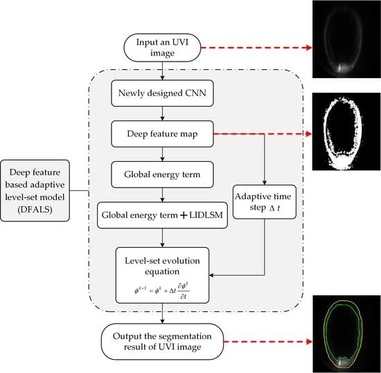
The flow diagram of our work is shown in Figure 2. First, the CNN designed in our work is trained on the training samples extracted from the UVI image data set. Following this, the global energy term and adaptive time step are devised based on the confidence value obtained from trained CNN. Subsequently, the global energy term and adaptive time-step are introduced into the LIDLSM for the extraction of the auroral oval. Experiments performed on the UVI image data sets demonstrate that the proposed method, compared with the state-of-the-art algorithms, can obtain more accurate segmentation results and is more robust to different contour initializations.

The remainder of the paper is organized as follows. The second section briefly reviews state-of-the-art level set models and previous level set models explicitly designed for auroral oval extraction, which include the SPFLIF-IS and LIDLSM. In Section 3, the global energy term and adaptive time step will be devised and introduced into the dual level set framework. The UVI data set, experimental results and analysis are presented in Section 4. Section 5 reports the conclusions.

2. Related Works

SPFLIF-IS [24] is a universally applicable image segmentation method, which combines the local fitted image formulation (LIF) [30] and the improved signed pressure force (SPF) [31] for inhomogeneous image segmentation.

By combining the improved SPF function with the LIF model, the level set evolution equation of SPFLIF-IS was defined as:

$$\frac{\partial \varphi }{\partial t}=\left(1-{\lambda }_1\right)·\alpha ·spf\left(I\left(u\right)\right)+{\lambda }_1\left(I-I^{LIF}\right)\left(I_{inner}-I_{outter}\right)\delta \left(\varphi \right)$$

(1)

The first term of Equation (1) is the product of the improved SPF ($spf\left(I\left(u\right)\right)$) and the balloon force ($\alpha$). The improved SPF function has values in the range $[-1,1]$. It modulates the signs of the pressure force inside and outside the region of interest so that the contour shrinks when outside the object, or expands when inside the object [32]. The second term is the level set evolution function corresponding to the LIF model, where $I_{inner}$ and $I_{outer}$ denote the mean grayscale intensity of $\left\{v|\varphi \left(v\right)>0,||v-u||<r\right\}$ and $\left\{v|\varphi \left(v\right)\le 0,||v-u||>r\right\}$, respectively. $I^{LIF}$ is the local fitted image and $\delta \left(\varphi \right)$ is the univariate Dirac function. By utilizing the local image information, the LIF model is able to segment images with intensity inhomogeneity [30]. The weight coefficient ${\lambda }_1$ is used to adjust the weight between the SPF function and the LIF model. Based on global and local image information, inhomogeneous images can be segmented quickly and accurately by SPFLIF-IS.

LIDLSM [26] is a level set method explicitly designed for auroral oval segmentation. In LIDLSM, Yang et al. [26] utilized dual level set function of ${\varphi }_1$ and ${\varphi }_2$ to obtain the inner and outer auroral oval boundaries, respectively. Suppose that $I:\Omega \subset R^2$ is an image domain, $I:\Omega \to R^2$ is the input auroral oval image. Two level set functions can divide the auroral oval image into three regions:

$$\{\begin{array}{c}{S}_1=\left\{u\in \Omega |{\varphi }_1\left(u\right)>0\right\}\\ S_2=\left\{u\in \Omega |{\varphi }_1\left(u\right)\le 0,{\varphi }_2\left(u\right)>0\right\}\\ S_3=\{u\in \Omega |{\varphi }_2\left(u\right)>0\}\end{array}$$

(2)

This can be shown in Figure 3.

Assuming that the distance between ${\varphi }_1$ and ${\varphi }_2$ follows the Gaussian distribution, Yang et al. [26] introduced the shape energy term into LIDLSM. Besides, the local information term was constructed to improve the segmentation performance in the low contrast region, and the regularization term was adopted to ensure the curve can evolve smoothly towards the auroral oval boundaries and inhibit small isolated regions. Combining these three terms, the total energy functional of LIDLSM was defined as:

$$\begin{array}{c}{E}_{LIDLSM}={\lambda }_2\underset{\mathrm{shape}\mathrm{energy}\mathrm{term}}{\underbrace{{{\displaystyle \int }}_{\Omega }^{}\frac{{(|{\varphi }_1\left(u\right)-{\varphi }_2\left(u\right)|-\mu )}^2}{2{\sigma }^2}du}}+{\lambda }_3\underset{\mathrm{regularization}\mathrm{term}}{\underbrace{{\displaystyle \sum }_{i=1}^2{{\displaystyle \int }}_{\Omega }^{}|\nabla H\left({\varphi }_i\left(u\right)\right)|du}}+\\ \underset{\mathrm{local}\mathrm{information}\mathrm{term}}{\underbrace{{\displaystyle \sum }_{i=1}^2{{\displaystyle \int }}_{\Omega }^{}\delta \left({\varphi }_i\left(u\right)\right){{\displaystyle \int }}_{\Psi }^{}H\left({\varphi }_i\left(v\right)\right){(I\left(v\right)-I_{inner})}^2+\left(1-H\left({\varphi }_i\left(v\right)\right)\right){(I\left(v\right)-I_{outer})}^{2}dvdu}}\end{array}$$

(3)

where $\mu$ and $\sigma$ are mean and standard deviation of distance between ${\varphi }_1$ and ${\varphi }_2$. $\Psi =\left\{v|||v-u||<r\right\}$ indicates a local region with radius $r$ at pixel $u$. $I_{inner}$ and $I_{outer}$ denotes the mean grayscale intensity $\left\{v|{\varphi }_i\left(v\right)>0,||v-u||<r\right\}$ and $\left\{v|{\varphi }_i\left(v\right)\le 0,||v-u||>r\right\}$, respectively. ${\lambda }_2$ and ${\lambda }_3$ are constant coefficients controlling the strength of the shape energy term and the regularization term.

To obtain an accurate segmentation result of the auroral oval, LIDLSM employs the LLSRHT results to serve as the initial contours of the level set. However, the auroral oval region cannot be identified accurately if the initial contour is far away from the boundaries. Figure 4c shows LIDLSM’ segmentation failure in such a case.

3. Deep Feature-Based Adaptive Level Set Model (DFALS)

To overcome the auroral oval segmentation problems brought by the image intensity inhomogeneity, the high noise level and the level set initialization, this work proposes a deep feature-based adaptive level set (DFALS) model with the aid of the convolutional neural network.

3.1. CNN Model Design

In deep learning, CNNs are the most popular networks used for image classification. In this work, CNN is utilized to obtain the confidence value of each pixel belonging to the auroral oval region. The design of the proposed CNN architecture is motivated by [33], and the structure is shown in Figure 5. This network consists of an input layer, four convolution layers, and two fully connected layers. The input layer specifies a sub-image extracted from the auroral images with the size of 11 × 11. Each convolutional layer has a 3 × 3 filter and a rectified linear unit (ReLU) [34], and zeros are padded around the border before each convolution so that the output does not lose relative pixel position information. The feature map (yellow) after the fourth convolutional layer is reduced to a one-channel feature as a 1 × 576 vector. The output of the network is a 1 × 2 vector which indicates the confidence values that the center pixel belongs to the auroral region (red) and background region (green).

The cross-entropy loss function [35] is adopted as the cost function for the network:

$$Loss=-[y\widehat{\log y}+\left(1-y\right)\log (1-\widehat{y})]$$

(4)

where $y$ denotes the sample label. If the center pixel of the sub-image locates in the auroral oval region, the sample label is 1; otherwise, the label is 0. $\widehat{y}$ is the confidence value, which indicates the probability that the center pixel belongs to the auroral oval region. The parameters of CNN are optimized by the back-propagation algorithm [36].

3.2. Constructing the Global Energy Term

Inspired by the sliding window method [37], we gather the sub-images (11 × 11 pixels) with stride equal 1 pixel horizontally and vertically from each UVI image. Since the auroral images used in this work have a fixed size of 228 × 200 as shown in Figure 6a, 45,600 sub-images with the size of 11 × 11 can be obtained after padding zeros at the border of each image. Taking each of the 45,600 sub-images as the input of the pre-trained CNN, we can obtain the confidence value $\widehat{y}$ ($\widehat{y}\in \left[0,1\right]$) of the center pixel in the sub-image, which reflects the probability of the pixel locating at the aurora oval region. All confidence values of the pixels in an image can be visualized through the deep feature map, whose gray value is $\widehat{I}=\widehat{y}\times 255$. An example of the auroral oval image and corresponding deep feature map are shown in Figure 6. With the deep feature map, we can detect the weak boundary regions of the aurora effectively.

Based on the deep feature map, we propose the global energy term as follows

$$E_{global}={{\displaystyle \int }}_{\Omega }^{}{(\widehat{I}\left(u\right)-{\widehat{c}}_1)}^{2}H\left({\varphi }_1\right)du+2{{\displaystyle \int }}_{\Omega }^{}{(\widehat{I}\left(u\right)-{\widehat{c}}_2)}^2\left(1-H\left({\varphi }_1\right)\right)H\left({\varphi }_2\right)du+{{\displaystyle \int }}_{\Omega }^{}{(\widehat{I}\left(u\right)-{\widehat{c}}_3)}^2\left(1-H\left({\varphi }_2\right)\right)du$$

(5)

${\widehat{c}}_1$, ${\widehat{c}}_2$ and ${\widehat{c}}_3$ represent the mean gray intensities of region $S_1$, $S_2$ and $S_3$ in the deep feature map, which can be calculated as:

$${\widehat{c}}_1=\frac{{{\displaystyle \int }}_{\Omega }\widehat{I}\left(u\right)H\left({\varphi }_1\right)du}{{{\displaystyle \int }}_{\Omega }H\left({\varphi }_1\right)du}{\widehat{c}}_2=\frac{{{\displaystyle \int }}_{\Omega }\widehat{I}\left(u\right)\left(1-H\left({\varphi }_1\right)\right)H\left({\varphi }_2\right)du}{{{\displaystyle \int }}_{\Omega }\left(1-H\left({\varphi }_1\right)\right)H\left({\varphi }_2\right)du}{\widehat{c}}_3=\frac{{{\displaystyle \int }}_{\Omega }\widehat{I}\left(u\right)\left(1-H\left({\varphi }_3\right)\right)du}{{{\displaystyle \int }}_{\Omega }1-H\left({\varphi }_3\right)du}$$

(6)

The global energy term contains three components. In the minimization of the global energy term, the first component can drive the inner level set (${\varphi }_1$) curve to evolve towards the inner boundary of the auroral oval, and the third component can drive the outer level set (${\varphi }_2$) curve to evolve towards the outer boundary. The second component can attract the inner and outer level set curves moving to the auroral oval boundary determined by the deep feature map simultaneously.

To obtain an accurate boundary of the auroral oval, we incorporate the global energy term into the LIDLSM, and the total energy functional of the DFALS can be formulated as

$$\begin{array}{ll}{E}_{DFALS}=& {\gamma }_1{{\displaystyle \int }}_{\Omega }^{}\frac{{(|{\varphi }_1\left(u\right)-{\varphi }_2\left(u\right)|-\mu )}^2}{2{\sigma }^2}du+{\gamma }_2{\displaystyle \sum }_{i=1}^2{{\displaystyle \int }}_{\Omega }^{}|\nabla H\left({\varphi }_i\left(u\right)\right)|du+{\gamma }_3·E_{global}\\ & {\displaystyle \sum }_{i=1}^2{{\displaystyle \int }}_{\Omega }^{}\delta \left({\varphi }_i\left(u\right)\right)\underset{\Psi }{{\displaystyle \int }}H\left({\varphi }_i\left(v\right)\right){(I\left(v\right)-I_{inner})}^2+\left(1-H\left({\varphi }_i\left(v\right)\right)\right){(I\left(v\right)-I_{outer})}^{2}dvdu\end{array}$$

(7)

Benefiting from the deep feature-based global energy term, the DFALS model can prevent the boundary leakage of the LIDLSM and obviously improve the segmentation accuracy at the low-contrast regions in the UVI images.

3.3. Constructing Adaptive Time-Step

It is worth noting that the confidence value $\widehat{y}$ also contains the positional information of the corresponding pixel. $\widehat{y}$ is relatively large if the pixel locates closely to the auroral oval region or even in it. Otherwise, $\widehat{y}$ is small when the pixel is far away from the auroral oval region.

As shown in Figure 4c, the segmentation failure is brought by the shape energy term of LIDLSM. More specifically, when the inner and outer level set curves cannot evolve to the adjacent region of the auroral oval simultaneously, the one far from the boundary attracts the other to continue evolving and overstepping the region of the auroral oval, which results in the segmentation failure eventually. The adaptive time step $\Delta t$ is proposed to address this problem. In this solution, the time step is large when the confidence value is small. Otherwise, the time step will be set with a low value or even zero.

According to these requirements, the adaptive time step can be designed as follows:

$$\Delta t=\{\begin{array}{cc}max(0,4{\widehat{y}}^2-8\widehat{y}+3),& k\le 300\\ 0.5,& k>300\end{array}$$

(8)

where $k$ refers to the $k^{th}$ iteration of the level set evolution. Auroral oval image and the corresponding time step map in the former 300 iterations are shown in Figure 7.

As shown by Figure 7, under the effect of the adaptive time step, the level set curve will slow down or even stop moving when approaching the nearby region of the auroral oval boundaries. Therefore, the adaptive time step can effectively prevent the contour curve from overstepping the auroral oval region and resulting in the segmentation failure. When $k>300$, the dual level set curves continue advancing with a relatively small and stable time step $\Delta t=0.5$.

3.4. Implementation of the DFALS

As aforementioned, the energy functional of the proposed method is defined as Equation (7). By introducing the time variable $t$ and minimizing the energy functional with respect to ${\varphi }_1$ and ${\varphi }_2$, we can deduce the following evolution equations for ${\varphi }_1$ and ${\varphi }_2$ by the gradient descent flow:

$$\begin{array}{ll}\frac{\partial {\varphi }_1\left(u\right)}{\partial t}=& {\gamma }_1\frac{\left(|{\varphi }_1\left(u\right)-{\varphi }_2\left(u\right)|-\mu \right)}{{\sigma }^2}+\delta \left({\varphi }_1\left(u\right)\right){{\displaystyle \int }}_{\Psi }^{}\delta \left({\varphi }_1\left(v\right)\right)({(I\left(v\right)-I_{inner})}^2-\left(I\left(v\right)-I_{outer}{)}^2\right)dv\\ & +{\gamma }_2\delta \left({\varphi }_1\left(u\right)\right)div(\frac{\nabla {\varphi }_1\left(u\right)}{|{\varphi }_1\left(u\right)|})+{\gamma }_3(\delta \left({\varphi }_1\left(u\right)\right)·((\widehat{I}\left(u\right)-{\widehat{c}}_1{)}^2-H({\varphi }_2)(\widehat{I}\left(u\right)-{\widehat{c}}_2{)}^2))\end{array}$$

(9)

$$\begin{array}{ll}\frac{\partial {\varphi }_2\left(u\right)}{\partial t}=& {\gamma }_1\frac{\left(|{\varphi }_1\left(u\right)-{\varphi }_2\left(u\right)|-\mu \right)}{{\sigma }^2}+\delta \left({\varphi }_2\left(u\right)\right){{\displaystyle \int }}_{\Psi }^{}\delta \left({\varphi }_2\left(v\right)\right)({(I\left(v\right)-v_{inner})}^2-\left(I\left(v\right)-v_{outer}{)}^2\right)dv\\ & +{\gamma }_2\delta \left({\varphi }_2\left(u\right)\right)div(\frac{\nabla {\varphi }_2\left(u\right)}{|{\varphi }_2\left(u\right)|})+{\gamma }_3(\delta ({\varphi }_2\left(u\right))·((\widehat{I}\left(u\right)-{\widehat{c}}_2{)}^2\left(1-H\left({\varphi }_1\right)\right)-(\widehat{I}\left(u\right)-{\widehat{c}}_3{)}^2))\end{array}$$

(10)

The evolution equation can be discretized as:

$${\varphi }^{k+1}={\varphi }^k+\Delta t\frac{\partial {\varphi }^k}{\partial t}$$

(11)

where $k$ refers to the $k^{th}$ iteration. The adaptive time step $\Delta t$ is introduced into the evolution equation.

The main procedures of the proposed DFALS model are summarized in Algorithm 1 as follows:

Algorithm 1. Deep feature-based adaptive level set model (DFALS).

Preprocessing: Train the CNN with the training samples, and then construct each UVI image’s corresponding deep feature map with the trained CNN.

Input: An original UVI image and the corresponding deep feature map

Output: The segmentation result of the auroral oval image

Step 1: Initialize the level set functions ${\varphi }_1$ and ${\varphi }_2$, and set the coefficient parameters ${\gamma }_1$, ${\gamma }_2$ and ${\gamma }_3$. Step 2: For$k=1:K$ ($K$ is the total number of iterations). Step 3: Calculate the gradient descent flow for ${\varphi }_1$ and ${\varphi }_2$ by Equations (9) and (10). The gradient descent flow of the shape energy term, the regularization term, and the local information term are calculated with the original UVI image, and the gradient descent flow of the global energy term is calculated with the corresponding deep feature map. Step 4: Calculate the adaptive time step according to Equation (8). Step 5: Calculate the level set evolution equation using Equation (11). Step 6: If the evolution of the curves is stable or the predetermined iteration number is reached, then output the segmentation result; otherwise, return to Step 4. Step 7: End for Step 8: Output the segmentation result.

4. Experiment and Results

4.1. UVI Data Set

The data set includes 200 auroral oval images which were captured by ultraviolet imager (UVI) aboard on National Aeronautics and Space Administration (NASA) Polar satellite on 10 January 1997, 31 July 1997, 15 January 1998, and 25 January 1998. The Polar satellite was launched in February 1996 into a highly elliptical orbit of 2 × 9$R_E$ (Earth radius) with 86° inclination, and it views the north polar region for about 9 hours out of every 18-hour orbit [38]. Auroral oval images used in this study were obtained using the Lyman–Birge–Hopfield ‘‘long’’ (LBHL) filter of the UVI on the Polar satellite, and the auroral radiance in this wavelength band originates from $N_2$ (Nitrogen molecules) emissions at altitudes of ~120 km [39]. The corresponding benchmark images which show the auroral oval region were annotated and cross-verified by several aurora experts manually. An example of the auroral oval image and the corresponding benchmark image is shown in Figure 8.

Among the UVI images, 50 typical images are used to extract training samples for CNN, and the rest 150 images are used as test images for the validation of the proposed method. As abovementioned, 45,600 sub-images with the size of 11 × 11 can be obtained from each UVI image, in which 4000 sub-images are used for training CNN. Therefore, there are 200,000 (4000 × 50) sub-images are selected as training samples for CNN. The process of training samples extraction is shown in Figure 9. In the first step, 2000 auroral oval pixels and 2000 background pixels are selected randomly from each image. In the second step, centered on these pixels, sub-images with the size of 11 × 11 are available. In the third step, the center pixels’ values in the benchmark image are taken as the labels of the corresponding sub-images. With the 200,000 training samples, the prediction accuracy reaches 93.2% when the CNN was trained for 50,000 epochs.

The 150 test images that do not participate in the training process are used for validating the performance of the DFALS method. The experimental results are also compared with other auroral oval segmentation models and recently developed level set methods, i.e., SIIALSM [25], LIDLSM [26], RLSF [23], and SPFLIF-IS [24]. The parameters of the DFALS are empirically set as follows: ${\gamma }_1=1$, ${\gamma }_2=2$, ${\gamma }_3=1$. Optimal parameters of other methods are chosen to guarantee the fairness of the comparison.

4.2. Robustness to Contour Initializations

We evaluate the influence of contour initializations on the segmentation results for the LIDLSM and DFALS models. The segmentation results of these two methods initialized by different level set curves are shown in Figure 10. Despite the differences among several initializations, the DFALS model yields accurate segmentation results. In contrast, the LIDLSM is extremely sensitive to the initial contour positions, which can be seen from its unreasonable segmentation results. Therefore, benefiting from the deep feature-based adaptive time step, the DFALS model shows stronger robustness to different contour initializations.

4.3. Comparison with Other Methods

To further testify the effectiveness and robustness of the DFALS model, two recently proposed universally applicable image segmentation methods (RLSF, SPFLIF-IS) and methods designed specifically for auroral oval segmentation (SIIALSM, LIDLSM), were conducted to compare with our method. The LLSRHT results were adopted as the initial level set contours of the SIIALSM and the LIDLSM to guarantee the fairness of comparison.

4.3.1. Subjective Evaluation

From test images for validating the DFALS model, we choose three auroral oval images that are difficult to segment for comparison experiments. In the experiments, the inner and outer level set curves of the DFALS model are initialized by two concentric circles, whose radius is 15 and 98, respectively. The center of concentric circles coincides with the image center. The contour initializations of different methods for these three auroral oval images are shown in Figures S1–S3.

As shown by the red rectangle in Figure 11a, there exist dayglow contamination regions in the first UVI image. The auroral oval annotated by experts and segmentation results obtained by different methods automatically are also shown in Figure 11b–f. The RLSF, SPFLIF-IS, and SIIALSM models mistakenly identify the edge of UVI’s lens as the outer boundary of the auroral oval. In contrast, LIDLSM and DFALS obtain reasonable segmentation results. Compared with the LIDLSM, the DFALS model shows superiority on retaining the details of the inner boundary of the auroral oval, as shown by the blue rectangle in Figure 11f,g.

The second auroral oval image contains low contrast region as marked by the red rectangle in Figure 12a. As aforementioned, the RLSF model improved the segmentation result when the image’s noise distribution is unknown and the SPFLIF-IS model was developed to address the segmentation problem brought by image intensity inhomogeneity. However, these two methods fail to obtain accurate segmentation results. The RLSF model eliminates the noise point in the segmentation result while missing to extract complete auroral oval in the low contrast region. The SPFLIF-IS model inhibits apparent boundary leakage of the auroral oval in the low contrast region yet regarding many noise pixels as the auroral oval region. Influenced by the intensity inhomogeneity, the segmentation results of SIIALSM and LIDLSM also breaks in the low contrast region. Compared with other methods, the DFALS model obtains the most reasonable segmentation result with the help of deep feature-based global energy term.

The third auroral oval image also includes low-contrast regions around the boundary, which is marked with the red box in Figure 13a. As seen from the segmentation results, the contours obtained by RLSF and SIIALSM break in the low contrast region, and SPFLIF-IS mistakes the noise pixels as part of the auroral oval. By comparing Figure 13b,f, we can conclude that although the boundary leakage does not appear in the segmentation result of LIDLSM, the extracted auroral oval deviates from the benchmark significantly in the low contrast region. However, regardless of the intensity inhomogeneity and image noise, DFALS yields the segmentation result that most closely matches the benchmark.

4.3.2. Objective Evaluation

To objectively evaluate the segmentation accuracy of different methods, an experiment was conducted to compare the segmentation results with the benchmark on 150 test images. Both boundary-based and region-based measures are employed.

• Boundary-based measurement

Pixel deviation $P_d$ and gap pixel percentage $P_g$ [19] are adopted as the evaluation metrics in the Boundary-based measurement. $P_d$ is a summative measure of the distance variation of the automatically segmented boundary from the expert’s annotated boundary. $P_g$ indicates the proportion of the gap in the whole auroral oval boundary. The smaller these two metric values, the better the segmentation result. $P_d$ and $P_g$ are calculated as follows:

$$P_d=\frac{{{\displaystyle \sum }}_{b_a\in B_a}d\left(b_a,B_b\right)+{{\displaystyle \sum }}_{b_b\in B_b}d\left(b_b,B_a\right)}{N_a+N_b}$$

(12)

$$P_g=\frac{N_{gap}}{N_b}\times 100\%$$

(13)

where $B_a$ and $B_b$ are the pixel sets on the segmented auroral oval boundaries and the benchmark boundaries. $b_a$ and $b_b$ are pixels in $B_a$ and $B_b$, respectively. $N_a$ and $N_b$ are the number of elements in set $B_a$ and $B_b$, respectively, and $N_{gap}$ denotes the number of gap pixels. $d\left(b_1,B_2\right)=\underset{b_2\in B_2}{min}{b}_1-b_2$ represents the minimum distance from pixel $b_1$ to the pixels in set $B_2$.

Table 1. The mean value and standard deviation of $P_d$ given by different methods on the test images.

Methods	RLSF	SPFLIF-IS	SIIALAM	LIDLSM	DFALS
Mean value	7.114	6.221	6.314	4.614	1.651
Standard deviation	3.456	3.401	8.354	8.063	1.289

and

Table 2. The mean value and standard deviation of $P_g$ given by different methods on the test images in %.

Methods	RLSF	SPFLIF-IS	SIIALAM	LIDLSM	DFALS
Mean value	3.010	0.200	1.142	0.600	0.100
Standard deviation	5.153	1.090	4.006	5.513	0.482

list the mean value and standard deviation of $P_d$ and $P_g$ given by different methods. The best results are labeled in bold. For these two metrics, the RLSF model performs slightly worse than the SPFLIF-IS model, which reflects that the problem of auroral oval segmentation is mainly brought by intensity inhomogeneity. Besides, the suboptimal $P_g$’s mean value of SPFLIF-IS shows that this method can efficiently inhibit the boundary leakage in the low contrast region in the UVI images. Both initialized by LLSRHT result, the comparison between the LIDLSM and the SIIALSM verifies the effectiveness of the shape energy term in the LIDLSM. Though the $P_d$’s mean value of the LIDLSM is suboptimal, this method owes the largest value of standard deviation except for SIIALSM. The large $P_d$’s standard deviation of the SIIALSM and LIDLSM is mainly brought by some poor LLSRHT result initializations, which also indirectly reflects that these two methods are sensitive to contour initializations.

• Region-based measurement

The percentage of mislabeled pixels $P_{mp}$ [19] measures the deviation of the automatically segmented auroral oval region ($R_a$) from the benchmark annotated by experts manually ($R_b$), and it is used as the metric for region-based measurement. $P_{mp}$ is calculated as the following formula.

$$P_{mp}=\frac{N_{miss}+N_{false}}{N_b+N_a}\times 100\%$$

(14)

where $N_{miss}$ represents the number of pixels in $R_b$ but not in $R_a$, $N_{false}$ is the number of pixels in $R_a$ but not in $R_b$.

The mean value and standard deviation of $P_{mp}$ given by different methods are listed in

Table 3. The mean value and standard deviation of $P_{mp}$ given by different methods on test images in %.

Methods	RLSF	SPFLIF-IS	SIIALSM	LIDLSM	DFALS
Mean value	31.173	33.927	33.002	25.484	16.565
Standard deviation	6.609	6.9569	17.729	6.610	3.560

, and the best results are labeled in bold. The $P_{mp}$’s mean value of SPFLIF-IS is the largest for the reason that this method mistakes many noise pixels as the auroral oval region, and the $P_{mp}$’s mean value of LIDLSM is suboptimal due to the effectiveness of its local information term. Compared with other methods, the standard deviation of $P_d$ and $P_{mp}$ obtained by the SIIALSM are the largest, which shows that this method is sensitive to different auroral oval shapes and contour initializations. The auroral oval region extracted by the DFALS model agrees well with the expert annotated auroral region which can be verified from the lowest $P_{mp}$’s mean value and standard deviation. Indeed, the DFALS model obtains the lowest value of all three metrics. From Table 3, we can conclude that with the help of deep feature-based global energy term, the auroral oval segmented by the DFALS matches well with the benchmark annotated by the experts.

5. Conclusions

In this paper, motivated by previous auroral oval segmentation methods, we propose a novel deep feature-based adaptive level set model to extract the auroral oval region in the UVI images. By utilizing the confidence value obtained from pre-trained CNN, the global energy term is constructed and incorporated into the LIDLSM’s energy functional. Additionally, an adaptive time step is introduced to the evolution equation of the level set. The experiments validate that the main contributions of our method are as follows:

• The comparative experiment between the LIDLSM and DFALS models demonstrate that the proposed method owes stronger robustness to different contour initializations.
• It can be seen from the subjective evaluation experiments that the auroral oval region extracted by DFALS agrees well with the experts’ annotated benchmark.
• Compared with the RLSF, SPFLIF-IS, SIIALSM, and LIDLSM models, the DFALS model improves the auroral oval segmentation accuracy in the intensity inhomogeneous region of the UVI images. Furthermore, the DFALS model also obtains the best performance in terms of the boundary- and region-based evaluation metrics.

The DFALS model focuses on segmenting the UVI images which have complete auroral oval. However, in practice, some aurora in the UVI images are incomplete due to the capturing position of the ultraviolet imager instrument aboard on the Polar satellite. In the future, we will consider adaptively setting the weight coefficients and introducing the prior knowledge of the auroral shape, so that the incomplete aurora can also be segmented accurately.

References

- Boudouridis, A.; Zesta, E.; Lyons, L.R.; Anderson, P.C.; Lummerzheim, D. Enhanced solar wind geoeffectiveness after a sudden increase in dynamic pressure during southward IMF orientation. J. Geophys. Res. Space Phys. 2005, 110. [Google Scholar] [CrossRef] [Green Version]
- Clausen, L.B.N.; Nickisch, H. Automatic Classification of Auroral Images From the Oslo Auroral THEMIS (OATH) Data Set Using Machine Learning. J. Geophys. Res. Space Phys. 2018, 123, 5640–5647. [Google Scholar] [CrossRef]
- Yang, Q.; Tao, D.; Han, D.; Liang, J. Extracting Auroral Key Local Structures From All-Sky Auroral Images by Artificial Intelligence Technique. J. Geophys. Res. Space Phys. 2019, 124, 3512–3521. [Google Scholar] [CrossRef] [Green Version]
- Akasofu, S.I. Dynamic morphology of auroras. Space Sci. Rev. 1965, 4, 498–540. [Google Scholar] [CrossRef]
- Lei, Y.; Shi, J.; Zhou, Y.; Tao, M.; Wu, J. Extraction of Auroral Oval Regions Using Suppressed Fuzzy C Means Clustering. In Proceedings of the International Geoscience and Remote Sensing Symposium, Valencia, Spain, 22–27 July 2018; pp. 6883–6886. [Google Scholar]
- Qian, W.; QingHu, M.; ZeJun, H.; ZanYang, X.; JiMin, L.; HongQiao, H. Extraction of auroral oval boundaries from UVI images: A new FLICM clustering-based method and its evaluation. Adv. Polar Sci. 2011, 22, 184–191. [Google Scholar] [CrossRef]
- Kvammen, A.; Gustavsson, B.; Sergienko, T.; Brändström, U.; Rietveld, M.; Rexer, T.; Vierinen, J. The 3-D Distribution of Artificial Aurora Induced by HF Radio Waves in the Ionosphere. J. Geophys. Res. Space Phys. 2019, 124, 2992–3006. [Google Scholar] [CrossRef]
- Ding, G.-X.; He, F.; Zhang, X.-X.; Chen, B. A new auroral boundary determination algorithm based on observations from TIMED/GUVI and DMSP/SSUSI. J. Geophys. Res. Space Phys. 2017, 122, 2162–2173. [Google Scholar] [CrossRef]
- Boudouridis, A.; Zesta, E.; Lyons, R.; Anderson, P.C.; Lummerzheim, D. Effect of solar wind pressure pulses on the size and strength of the auroral oval. J. Geophys. Res. Space Phys. 2003, 108. [Google Scholar] [CrossRef]
- Zhao, X.; Sheng, Z.; Li, J.; Yu, H.; Wei, K. Determination of the “wave turbopause” using a numerical differentiation method. J. Geophys. Res. Atmos. 2019, 124, 10592–10607. [Google Scholar] [CrossRef]
- Shi, J.; Wu, J.; Anisetti, M.; Damiani, E.; Jeon, G. An interval type-2 fuzzy active contour model for auroral oval segmentation. Soft Comput. 2017, 21, 2325–2345. [Google Scholar] [CrossRef]
- Kauristie, K.; Weygand, J.; Pulkkinen, T.I.; Murphree, J.S.; Newell, P.T. Size of the auroral oval: UV ovals and precipitation boundaries compared. J. Geophys. Res. 1999, 104, 2321. [Google Scholar] [CrossRef]
- Hu, Z.-J.; Yang, Q.-J.; Liang, J.-M.; Hu, H.-Q.; Zhang, B.-C.; Yang, H.-G. Variation and modeling of ultraviolet auroral oval boundaries associated with interplanetary and geomagnetic parameters. Space Weather 2017, 15, 606–622. [Google Scholar] [CrossRef]
- Meng, C.-I. Polar Cap Variations and the Interplanetary Magnetic Field; Springer: Dordrecht, The Netherlands, 1979; pp. 23–46. [Google Scholar]
- Liou, K.; Newell, P.T.; Sibeck, D.G.; Meng, C.-I.; Brittnacher, M.; Parks, G. Observation of IMF and seasonal effects in the location of auroral substorm onset. J. Geophys. Res. Space Phys. 2001, 106, 5799. [Google Scholar] [CrossRef] [Green Version]
- Hardy, D.A.; Burke, W.J.; Gussenhoven, M.S.; Heinemann, N.; Holeman, E. DMSP/F2 electron observations of equatorward auroral boundaries and their relationship to the solar wind velocity and the north-south component of the interplanetary magnetic field. J. Geophys. Res. Space Phys. 1981, 86, 9961–9974. [Google Scholar] [CrossRef]
- Meng, Y.; Zhou, Z.; Liu, Y.; Luo, Q.; Yang, P.; Li, M. A prior shape-based level-set method for auroral oval segmentation. Remote Sens. Lett. 2019, 10, 292–301. [Google Scholar] [CrossRef]
- Li, X.; Ramachandran, R.; He, M.; Movva, S.; Rushing, J.A.; Graves, S.J.; Lyatsky, W.B.; Tan, A. Comparing different thresholding algorithms for segmenting auroras. In Proceedings of the International Conference on Information Technology Coding and Computing, Las Vegas, NV, USA, 5–7 April 2004; pp. 594–601. [Google Scholar]
- Cao, C.; Newman, T.S. New shape-based auroral oval segmentation driven by LLS-RHT. Pattern Recognit. 2009, 42, 607–618. [Google Scholar] [CrossRef]
- Liu, H.; Gao, X.; Han, B.; Yang, X. An Automatic MSRM Method with a Feedback Based on Shape Information for Auroral Oval Segmentation. In Proceedings of the International Conference on Intelligent Science and Big Data Engineering, Beijing, China, 31 July–2 August 2013; pp. 748–755. [Google Scholar]
- Kass, M.; Witkin, A.; Terzopoulos, D. Snakes: Active contour models. Int. J. Comput. Vis. 1988, 1, 321–331. [Google Scholar] [CrossRef]
- Sun, L.; Meng, X.; Xu, J.; Zhang, S. An Image Segmentation Method Based on Improved Regularized Level Set Model. Appl. Sci. 2018, 8, 2393. [Google Scholar] [CrossRef] [Green Version]
- Niu, S.; Qiang, C.; Sisternes, L.D.; Ji, Z.; Rubin, D.L. Robust noise region-based active contour model via local similarity factor for image segmentation. Pattern Recognit. 2016, 61, 104–119. [Google Scholar] [CrossRef] [Green Version]
- Sun, L.; Meng, X.; Xu, J.; Tian, Y. An Image Segmentation Method Using an Active Contour Model Based on Improved SPF and LIF. Appl. Sci. 2018, 8, 2576. [Google Scholar] [CrossRef] [Green Version]
- Yang, X.; Gao, X.; Li, J.; Han, B. A shape-initialized and intensity-adaptive level set method for auroral oval segmentation. Inf. Sci. 2014, 277, 794–807. [Google Scholar] [CrossRef]
- Yang, P.; Zhou, Z.; Shi, H.; Meng, Y. Auroral oval segmentation using dual level set based on local information. Remote Sens. Lett. 2017, 8, 1112–1121. [Google Scholar] [CrossRef]
- Ham, Y.-G.; Kim, J.-H.; Luo, J.-J. Deep learning for multi-year ENSO forecasts. Nature 2019, 573, 568–572. [Google Scholar] [CrossRef] [PubMed]
- Silver, D.; Schrittwieser, J.; Simonyan, K.; Antonoglou, I.; Huang, A.; Guez, A.; Hubert, T.; Baker, L.; Lai, M.; Bolton, A.; et al. Mastering the game of Go without human knowledge. Nature 2017, 550, 354. [Google Scholar] [CrossRef]
- Girshick, R. Fast R-CNN. In Proceedings of the IEEE International Conference on Computer Vision, Santiago, Chile, 7–13 December 2015; pp. 1440–1448. [Google Scholar]
- Zhang, K.; Song, H.; Zhang, L. Active contours driven by local image fitting energy. Pattern Recognit. 2010, 43, 1199–1206. [Google Scholar] [CrossRef]
- Abdelsamea, M.M.; Tsaftaris, S.A. Active contour model driven by Globally Signed Region Pressure Force. In Proceedings of the 2013 18th International Conference on Digital Signal Processing (DSP), Santorini, Greece, 1–3 July 2013; pp. 1–6. [Google Scholar]
- Zhang, K.; Zhang, L.; Song, H.; Zhou, W. Active contours with selective local or global segmentation: A new formulation and level set method. Image Vis. Comput. 2010, 28, 668–676. [Google Scholar] [CrossRef]
- Kim, J.; Nguyen, D.; Lee, S. Deep CNN-Based Blind Image Quality Predictor. IEEE Trans. Neural Netw. Learn. Syst. 2018, 1–14. [Google Scholar] [CrossRef]
- Nair, V.; Hinton, G.E. Rectified Linear Units Improve Restricted Boltzmann Machines. In Proceedings of the International Conference on International Conference on Machine Learning, Haifa, Israel, 21–24 June 2010; pp. 807–814. [Google Scholar]
- de Boer, P.-T.; Kroese, D.P.; Mannor, S.; Rubinstein, R.Y. A Tutorial on the Cross-Entropy Method. Ann. Oper. Res. 2005, 134, 19–67. [Google Scholar] [CrossRef]
- Rumelhart, D.; Hinton, G.; Williams, R. Learning Internal Representation by Back-Propagation Errors. Nature 1986, 323, 533–536. [Google Scholar] [CrossRef]
- Drożdż, M.; Kryjak, T. FPGA Implementation of Multi-scale Face Detection Using HOG Features and SVM Classifier. Image Process. Commun. 2017, 21, 27–44. [Google Scholar] [CrossRef] [Green Version]
- Brittnacher, M.; Spann, J.; Parks, G.; Germany, G. Auroral observations by the polar Ultraviolet Imager (UVI). Adv. Space Res. 1997, 20, 1037–1042. [Google Scholar] [CrossRef]
- Carbary, J.F. Auroral boundary correlations between UVI and DMSP. J. Geophys. Res. 2003, 108, 1018. [Google Scholar] [CrossRef] [Green Version]
Figure 1.
Aurora images. (a) Aurora images captured by ultraviolet imager (UVI). (b) Aurora images captured by all-sky imagers (ASI).
Figure 2.
The flow diagram of the deep feature-based adaptive level set (DFALS) model.
Figure 3.
The three regions divided by and .
Figure 4.
The auroral oval image and the local information based dual level set auroral oval segmentation method’s (LIDLSM’s) segmentation results obtained by different initializations. (a) The original auroral oval image (top) and image after histogram equalization (bottom) which can show the auroral structure more clearly. (b) The linear least square randomized Hough transform method (LLSRHT) based initialization (top) and segmentation result of LIDLSM (bottom). (c) The self-defined initialization that initial level set curves are far away from auroral oval boundaries (top) and low-precision segmentation result of LIDLSM (bottom).
Figure 5.
Convolutional neural network (CNN) architecture. “Conv” and “FC” indicate convolutional layers and fully connected layers, respectively.
Figure 6.
Auroral oval image and the corresponding deep feature map. (a) Auroral oval image. (b) The corresponding deep feature map.
Figure 7.
Auroral image and the corresponding time step map. (a) Auroral oval image. (b) The corresponding time step map.
Figure 8.
Auroral oval image and the corresponding benchmark image. (a) Auroral oval image. (b) Benchmark image.
Figure 9.
Extract training samples from the auroral oval images.
Figure 10.
The segmentation results of LIDLSM and the deep feature-based adaptive level set (DFALS) model initialized by several different level set curves. (a) The UVI images captured by Polar satellite on Jul 31 1997 01:34:00 and Jul 31 1997 01:47:23. (b) The initial level set curves. (c) Segmentation results of the DFALS. (d) Segmentation results of the LIDLSM.
Figure 11.
The segmentation results of different methods. (a) UVI image captured by the Polar satellite on Jul 31 1997 09:34:48. (b) The benchmark annotated by experts manually. (c) The segmentation result of the region-based active contour model via local similarity factor (RLSF). (d) The segmentation result of the improved signed pressure force and local image fitting based image segmentation (SPFLIF-IS) method. (e) The segmentation result of the shape-initialized and intensity-adaptive level set method (SIIALSM). (f) The segmentation result of LIDLSM. (g) The segmentation result of DFALS.
Figure 12.
The segmentation results of different methods. (a) UVI image captured by polar satellite on Jan 10 1997 01:16:40. (b) The benchmark annotated by experts manually. (c) The segmentation result of RLSF. (d) The segmentation result of SPFLIF-IS. (e) The segmentation result of SIIALSM. (f) The segmentation result of LIDLSM. (g) The segmentation result of DFALS.
Figure 13.
The segmentation results of different methods. (a) UVI image captured by polar satellite on Jan 10 1997 03:10:08. (b) The benchmark annotated by experts manually. (c) The segmentation result of RLSF. (d) The segmentation result of SPFLIF-IS. (e) The segmentation result of SIIALSM. (f) The segmentation result of LIDLSM. (g) The segmentation result of DFALS.