
Optimization of Linear Quantization for General and Effective Low Bit-Width Network Compression

1
School of Computer Engineering & Science, Shanghai University, Shanghai 200444, China
2
Shanghai Engineering Research Center of Intelligent Computing System, Shanghai University, Shanghai 200444, China
*
Author to whom correspondence should be addressed.
†
These authors contributed equally to this work.
Algorithms 2023, 16(1), 31; https://doi.org/10.3390/a16010031
Submission received: 7 December 2022
/
Revised: 23 December 2022
/
Accepted: 27 December 2022
/
Published: 4 January 2023
Abstract
:Current edge devices for neural networks such as FPGA, CPLD, and ASIC can support low bit-width computing to improve the execution latency and energy efficiency, but traditional linear quantization can only maintain the inference accuracy of neural networks at a bit-width above 6 bits. Different from previous studies that address this problem by clipping the outliers, this paper proposes a two-stage quantization method. Before converting the weights into fixed-point numbers, this paper first prunes the network by unstructured pruning and then uses the K-means algorithm to cluster the weights in advance to protect the distribution of the weights. To solve the instability problem of the K-means results, the PSO (particle swarm optimization) algorithm is exploited to obtain the initial cluster centroids. The experimental results on baseline deep networks such as ResNet-50, Inception-v3, and DenseNet-121 show the proposed optimized quantization method can generate a 5-bit network with an accuracy loss of less than 5% and a 4-bit network with only 10% accuracy loss as compared to 8-bit quantization. By quantization and pruning, this method reduces the model bit-width from 32 to 4 and the number of neurons by 80%. Additionally, it can be easily integrated into frameworks such as TensorRt and TensorFlow-Lite for low bit-width network quantization.
1. Introduction
Due to their excellent data representation and feature learning ability, DNNs (deep neural networks) have achieved great success in a large number of tasks such as image classification, object detection, speech synthesis, and industrial and medical fields [1]. For example, Sallam et al. applied a DNN to speed control of three-phase induction [2] and blood diseases detection [3]. Their application scope has been extended to edge devices [4]. DNNs are high-complexity models that require huge energy consumption and memory cost. Due to factors such as security, privacy (e.g., medical data and industrial data), and latency (e.g., smart sensors, wearables, autopilot, and UAV tracking), inference of DNNs must be performed on edge devices, but the available computing resources are limited and subjected to strict power constraints [5]. Therefore, how to reduce the computation and storage while maintaining the accuracy of neural networks is a key issue in energy-sensitive applications. A fundamental way to decrease energy consumption and memory cost is to compress networks into lightweight models through pruning and quantization.
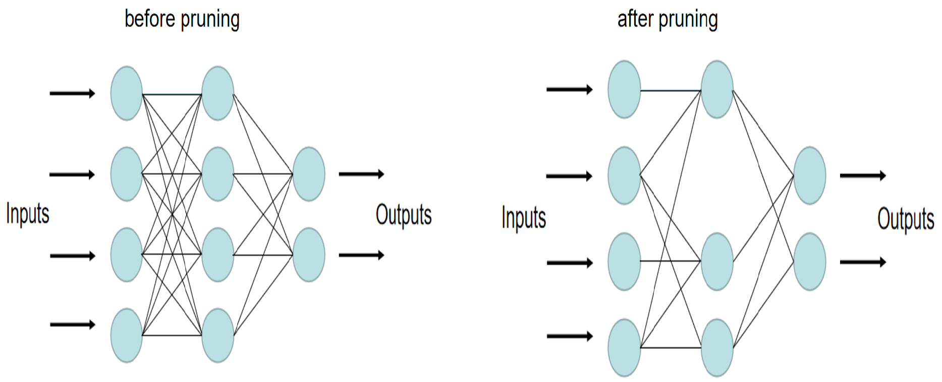
In practice, quantization usually needs to be done after the models are first “slimmed” down by pruning to obtain an effective lightweight model because neural networks are often over-parameterized. In 2015, Han et al. proved that reasonable pruning would not affect the accuracy of the neural networks [4]. Pruning can reduce a large pre-trained model into a smaller model without retraining [6]. Figure 1 depicts the basic inference process of the neural network. Each neuron connects through synapses with multiple neurons on the upper layer and needs to perform multiple floating-point operations. However, a large part of weights, i.e., the synapses, is redundant in the neural network. Not all operations will affect the reasoning ability of the network. Maarif et al. trained the model through structural learning with forgetting (SLF), eliminating weak connections between neurons during training and revealing the most influential injection molding parameters, while the performance of the model did not decline significantly [7].
Through pruning, the weight matrix can be converted into a sparse matrix and then many calculation tricks can be applied to improve the inference delay [8]. Pruning may result in a structured or unstructured network [6]. Unstructured pruning can prune any weight and can be considered fine-grained pruning. Compared with structured pruning, it does not generate irregular matrices while maintaining higher accuracy. This paper focuses on DNN weight quantization, which pays more attention to the accuracy of the model before and after pruning. Therefore, this paper will use fine-grained pruning to pre-process the model.
After the model is pruned, it can be further “slimmed” by converting floating-point weights into low-precision values through quantization. The quantized neural network has been proven to achieve a significant inference acceleration without a major drop in accuracy [9]. There are several types of quantization schemes according to the different quantization bit-widths. For example, Courbariaux et al. proposed BNNs (binary neural networks) to replace floating-point weights with 1 bit [10]. Rastegari et al. proposed to use XNOR-Net to quantify both activation and weight to 1 bit based on BNN [11]. Li et al. proposed TWNs (ternary weight networks) to quantize the weights into 2-bit weights [12]. In general, binary and ternary quantization schemes are associated with a specific network and have no generality. This paper endeavors to develop an effective quantization method that applies to general neural networks.
The quantization methods of DNN can be classified into two types: quantization aware training and post-training quantization. Quantization-aware training is to fine-tune the pre-trained model employing backpropagation when the floating-point weights are converted into fixed-point numbers [13]. Quantization-aware training can more effectively ensure accuracy, but it may not be practicable because it requires full datasets, and retraining and adjusting the model is time-consuming. On the other hand, post-training quantization only needs part of the training set.
Post-training quantization initially focused on 8-bit quantization, among which linear quantization is more commonly used. In 2017, TensorFlow-Lite, an automatic quantification tool that enabled on-device machine learning developed by Google, used linear quantization to automatically convert floating-point weights to 8-bit weights [13]. In the same year, NVIDIA developed the TensorRT tool which also applied linear quantization to create lightweight models. Due to the redundancy of network parameters and relatively large data representation space, 8-bit linear quantization usually does not cause a significant drop in model accuracy [13].
Currently, numerous edge devices may contain customizable parts such as FPGA, CPLD, and ASIC, to support adders and multipliers to do calculations on low bit-width weights. Using fewer bits to represent weights, model inference can directly simplify implementation and speed up execution in a hardware-friendly way [14]. However, post-training quantization with low bit-width usually results in a significant drop in accuracy. With traditional linear quantization, when the bit-width is under five, the model accuracy may drop to 1%.
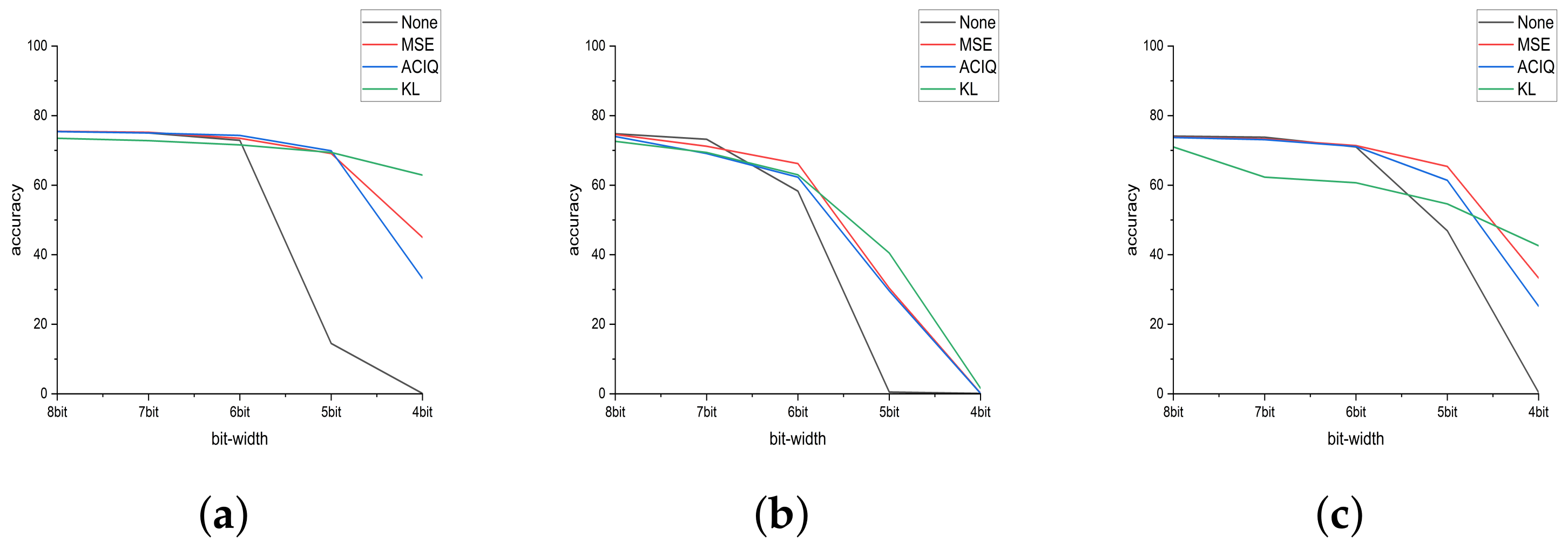
To deal with the above problem, researchers proposed to clip outliers because they generally believed that outliers in the network weights affect the results of quantization at low bit-widths [9]. For example, NVIDIA uses KL (Kullback–Leibler) divergence to reduce weight outliers in its TensorRT [15]. Figure 2 shows that quantization work based on the cropping method can reduce the accuracy drop, but still performs poorly on some models.
Different from previous studies, this paper looks deeply into the process of linear quantization of network weights. Linear quantization can be considered as two stages, clustering and mapping. In the clustering stage, the weights are divided into different categories through a uniform partition. In the mapping stage, the weights in each clustered category are mapped to one fixed-point number corresponding to its maximum and minimum. The fundamental reason for the reduction of the network accuracy by traditional linear quantization is that it combines the two stages into one stage, and at low bit-widths, it cannot accurately distinguish the categories of weights according to their true distribution. To overcome the challenges, this paper proposes a two-stage quantization method to optimize the clustering function of linear quantization thus promoting the effect of low bit-width network compression.
The motivation for this paper comes from a new understanding of the quantization process. To our best knowledge, this paper is the first to split the quantization process into two stages, clustering and mapping. To present a comprehensive study on post-training quantization, we also evaluate the result between clip threshold techniques and ours.
The main contributions of this paper are:
- This paper optimizes the linear quantization method with a two-stage technique. The clustering function is separated before mapping from the traditional linear quantization. Specifically, the optimized method applies a modified K-means algorithm to cluster the weights and then uses the uniform partition to map the centroids to fixed-point numbers.
- The results of the K-means algorithm are greatly affected by the initial cluster centroids, which may cause non-convergence. In neural network quantization, the number of cluster centroids can be determined by the bit-width. This paper selects the particle swarm algorithm to obtain the initial cluster centroids to facilitate the convergence of clustering.
- To reduce effectively both the energy consumption and memory cost of DNN models, models are first fine-grained pruning before quantization with low bit-width. The experimental results show that fine-grained pruning does not affect the accuracy of the quantized model. It is safe and necessary to perform pruning before quantization.
2. Related Work
2.1. Fine-Grained Pruning
Recently, neural network pruning is an important technique for reducing memory consumption and bandwidth. Pruning can help neural networks to be deployed in hardware resource-constrained environments. As described in Section 1, fine-grained pruning will be used in this paper to maintain the accuracy of the pruned model.
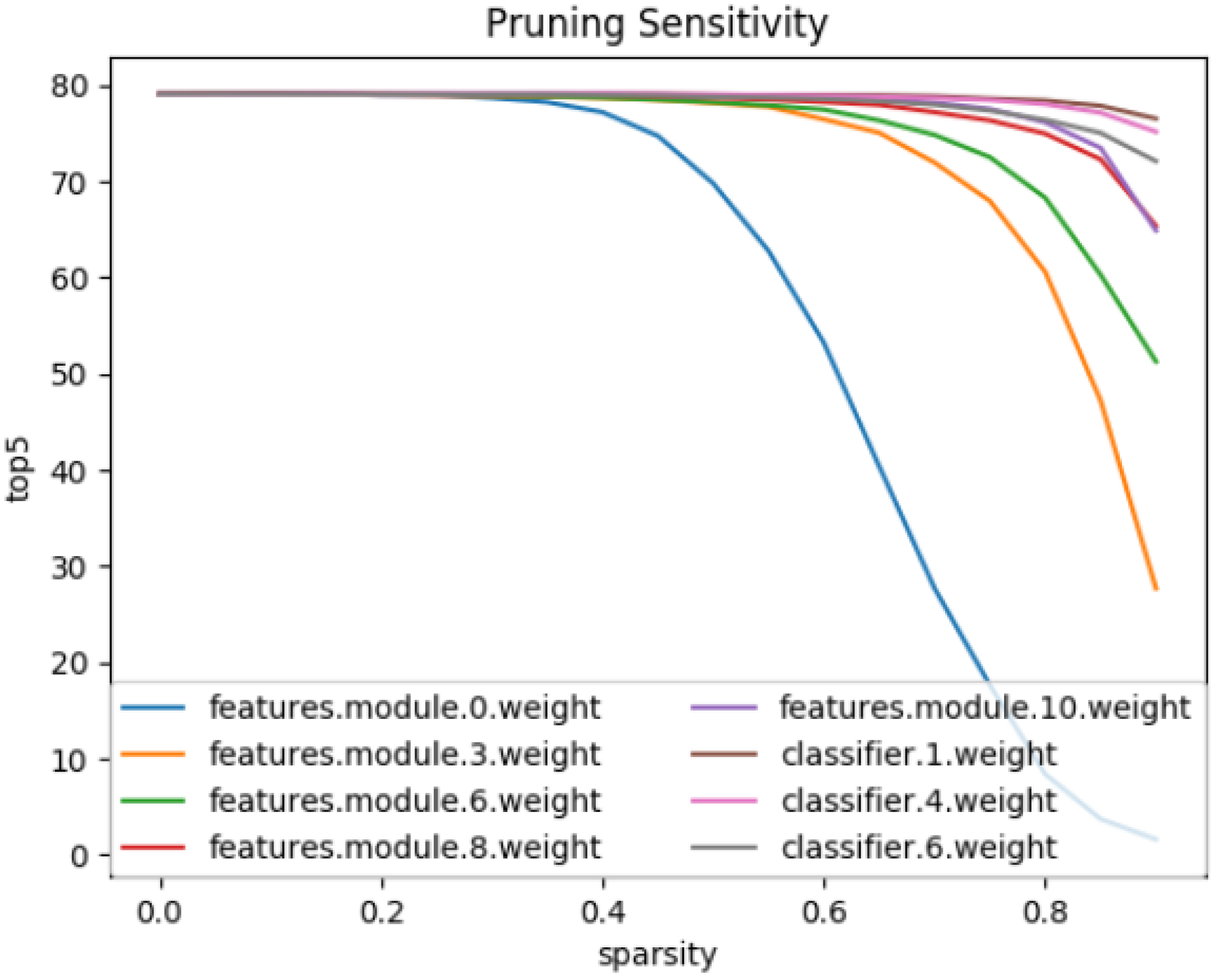
The fine-grained pruning method is generally threshold-based. The specific threshold needs to be carefully selected according to the weight of each layer. The different sparsities of the neural network will directly affect the accuracy of the network as shown in Figure 3. Han et al. used the tensor standard deviation as a threshold to prune the model [16].
Neural network pruning can be performed in multiple ways as static pruning and dynamic pruning according to whether retraining is required. Zhu et al. proposed AGP (automated gradual pruner), which automatically and gradually pruned the smallest weights according to the preset network sparsity, and then continuously fine-tuned the existing weights through training [8]. This method did not require many hyperparameter adjustments or any assumptions about the structure of the network or its constituent layers. This paper will use AGP-based unstructured pruning to prune the pre-trained model.
2.2. Post-Training Quantization
Past work on post-training quantization can be distinguished into three categories: weight-sharing quantization, uniform-partition quantization, and logarithmic quantization. Miyashita D et al. used logarithmic operations to quantify floating-point numbers into fixed-point numbers [18]. Unlike linear quantization, its quantization method is based on exponents. The weight matrix stores the value of exponents to achieve the effect of approximating fixed-point numbers. Logarithmic quantization accelerates inference through shift operations but requires specialized hardware support. This paper will mainly discuss weight-sharing quantization and uniform-partition quantization.
2.2.1. Weight-Sharing Quantization
For neural networks, weights can be clustered and shared. The majority of the literature on weight-sharing quantization aggregates weights into different sets to reduce memory space usage. Among them, weight aggregation is mainly based on clustering or hash functions. Chen et al. proposed HashedNet, which uses the hash function to randomly group weights into hash bushets, and the weights in the same hash bushet share the same value [19]. Clustering is the process that divides objects into multiple sets according to their characteristics. Clustering is usually used to compress network models. Han et al. used the K-means algorithm to cluster the network weights, and the weight matrix stored the labels of the clusters, and then processed the labels with the Huffman coding to compress the neural network model by more than 30 times, and the accuracy of the network did not drop significantly [4]. Wu et al. proposed a Q-CNN (quantized convolutional neural network) framework for compression by the K-means algorithm and then accelerated by the matrix factorization method [20].
Most of the research mentioned above stores the cluster labels instead of the cluster centroids to maximize the compression of the neural network model. However, in the actual inference, they still need to look up the table to get the cluster centroids the cluster labels still need to be converted into cluster centers, which cannot speed up the inference. Instead, this paper applies the clustering to the traditional linear quantization, and the neural network is compressed and quantized in fix-point numbers at the same time.
2.2.2. Uniform Partition Quantization
Uniform partition quantization is also known as linear quantization. Linear quantization refers to the use of max and min to scale the weights from floating-point values to fixed-point values. As mentioned above, Google and Nvidia developed TensorFlow-Lite and the TensorRt based on 8-bit linear quantization. One of the reasons their tools do not support lower-bit quantization is that the accuracy of low-bit quantization cannot be maintained.
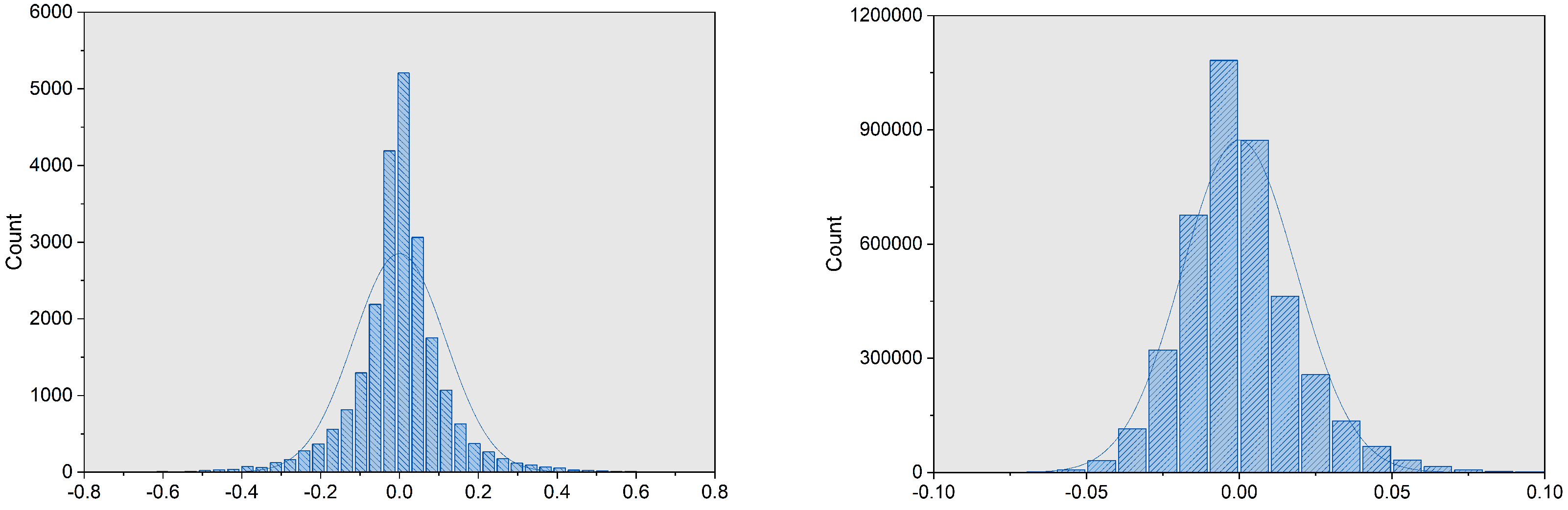
The researchers believe that the outliers of the network affect the results. The weights show a bell-shaped distribution as shown in Figure 4, most of the weights are located near 0, and a small part of the weights are distributed on both sides of the bell. Due to this distribution, in the case of low bit-widths, it will affect the result of uniform partition, and the accuracy of inference cannot be guaranteed. Therefore, the researchers proposed many schemes to prune the outliers. Shin et al. used pruning to deal with the weights, performed sensitivity analysis on each layer, pruned the weights according to the threshold, and finally used linear quantization to convert the weights into fixed-point numbers [21]. Banner et al. also used the pruning method to clip the outliers. Unlike Shin et al., they used the L2 norm method that minimizes the quantization error to determine the pruning threshold of each layer [22]. Similarly, they used linear quantization to convert the weights into fixed values. Unlike the existing clip-based methods, Zhao et al. proposed the method of OCS (outlier channel splitting) which split channels into a layer to reduce the magnitude of outliers, making the distance between the outlier and the center value closer, and finally, through using linear quantization, converted the model to a fixed-point model [23].
The methods mentioned in the above studies are all based on clipping, through compressing the max and min ranges of the weights to deal with the problem that linear quantization cannot distinguish weights at low bit-widths and then use linear quantization to convert the weights into fixed-point values. The biggest difference between the previous work and this paper is that the conclusion drawn in this paper is that the essence of linear quantification is a combination of clustering and scaling, as shown in Figure 4, and neural networks exhibit a bell-shaped distribution. Weights on either side of the bell affect the accuracy of linear quantization at low bit-widths, so this paper focuses on the optimization of the clustering function. The process of linear quantization can be equivalent to a clustering that uses the result of uniform partition as the initial point of clustering but has not been iteratively optimized. Therefore, an obvious method is to replace the uniform partition by using a clustering algorithm to cluster the weights before linear quantization. Linear quantization itself only plays the role of converting floating-point values into fixed-point values to avoid the problem of indistinguishable weights.
2.3. Metaheuristic
The term “metaheuristic” was first used by Glover [24] and is derived from two Greek words, meta and heuristic. Heuristic comes from the verb “heuriskein”, which means to find. The prefix meta means “beyond”, that is, to surpass at a higher level. The metaheuristic is a set of high-level strategies for exploring the search space using different heuristic algorithms.
Researchers have mapped the optimal behavior of living things, physical phenomena, and processes, behaviors based on social interactions to come up with optimization algorithms [25]. In 1992, Dorigo proposed the ant algorithm (AA) [26]. In 1995, Kennedy and Eberhart proposed particle swarm optimization (PSO) [27]. In recent years, some well-known evolution/swarm-based metaheuristics have also been developed. In 2019, Jain et al. proposed the squirrel search algorithm (SqSA) based on the foraging behavior of flying squirrels [28]. In 2020, Zhao et al. proposed manta ray foraging optimization (MRFO) based on the intelligent foraging behavior of manta rays [29].
Metaheuristic algorithms can find the global optimal solution and can be combined with other algorithms such as PSO and K-means. The combination of PSO and the K-means algorithm can solve the problem of unstable results of the K-means algorithm. The remainder of this study will show how this hybrid clustering optimizes quantization.
3. Two-Stage Quantization Method
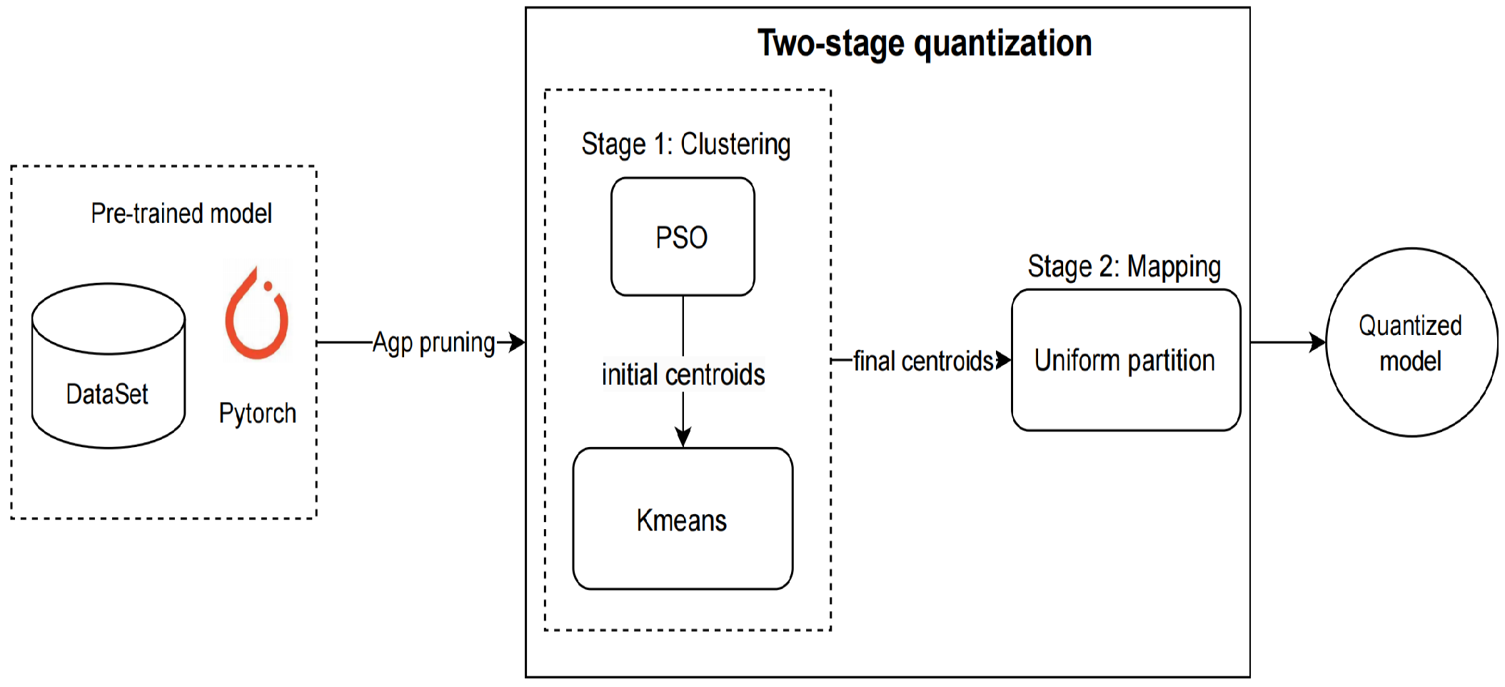
In this section, an optimized linear quantization for a low bit-width network is proposed. This method includes explicitly two stages: clustering and mapping, as shown in Figure 5. The “Hybrid clustering" module takes as input for a fine-grained pruned model which is pre-trained by PyTorch or other deep learning frameworks. It uses PSO-K-means to cluster the weights on each layer according to the preset bit-width. The mapping module maps the floating-point weights in each clustered set into one same fixed-point number according to its max and min ranges through the uniform partition algorithm. Details of this method will be explained in the following sub-sections.
3.1. Pruning
Our objective is that the model maintains a high test accuracy before and after pruning. To achieve this, the model will be pruned by the AGP (automated gradual pruner) algorithm before being quantized. AGP was proposed by the Distiller framework [17] for pruning neural networks.
For this paper, we define the following symbols:
- denotes the target sparsity;
- denotes the initial sparsity;
- denotes the current sparsity.
The original work is to set the target sparsity based on empirical values. This paper extends the calculation method of target sparsity . According to the three sigma guidelines, about 68% of the data in a normally distributed tensor are less than its standard deviation. Therefore, in this paper, the standard deviation of the weights tensor is used as a threshold magnitude to calculate the target sparsity .
3.2. Clustering
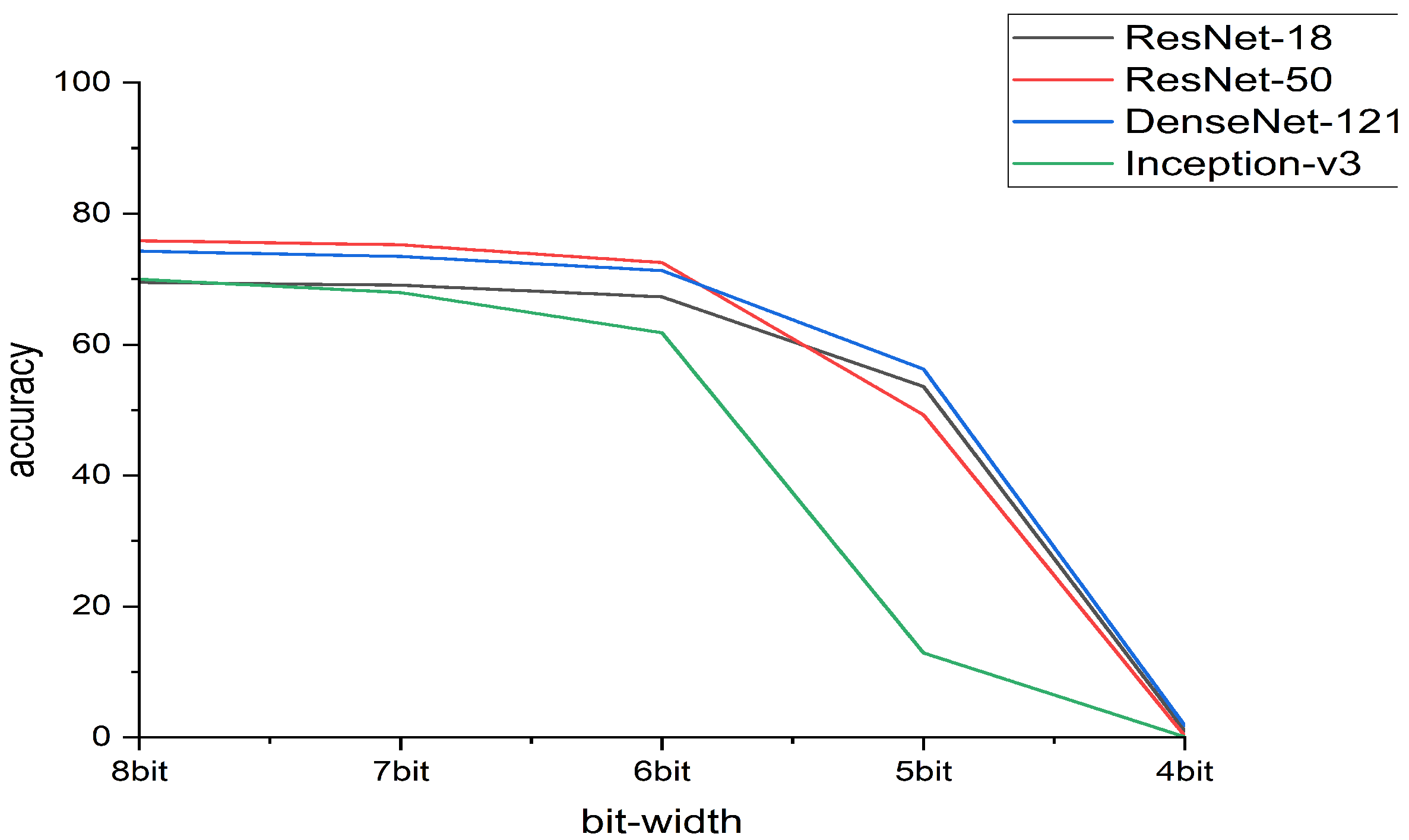
Data clustering is the process of grouping similar data vectors into multiple sets. Recently, clustering algorithms have been applied to a wide range of problems, including model compression and data analysis. This paper first presents application clustering for the optimization of quantization algorithms. Due to the bell-shaped distribution of the network weights, the uniform partition of the traditional linear quantization cannot distinguish the weights located in the middle part of the number axis when the bit-width is smaller than 5 bits, resulting in a significant decrease in the accuracy of the neural network. As shown in Figure 6, the accuracy of the model will have a huge decrease when the quantization bit-width is under 5 bits. This paper uses K-means to cluster the weights of each layer of the pre-training network so that the cluster set will not be changed when mapping.
3.2.1. K-Means
K-means is a simple yet often effective algorithm for clustering. This algorithm has a high degree of interpretability and a relatively fast convergence speed. It only needs to adjust the number of centroids. For neural network quantization, the number of centroids is determined according to the quantization bit-width. Its basic idea is that for a given dataset , the number of centroids K is calculated according to the bit-width, and the Euclidean distance is used as the similarity measurement. As shown in Equation (2), where are the centroid sets, the dataset is divided into K clusters, and the centroids are updated iteratively.
For this paper, we define the following symbols:
- denotes the i-th weight;
- denotes the centroid of cluster j;
- is the subset of weights that form cluster j.
As described in Algorithm 1, the cluster centroids need to be initialized before the K-means algorithm starts. The results of the K-means algorithm are not stable and are greatly affected by the initial cluster centroids and outliers. Thus, a reasonable initialization scheme needs to be selected. This paper examines three methods to initialize cluster centroids:
- (1)
- Random initialization;
- (2)
- Uniform partition;
- (3)
- Initialize by the optimization algorithm.
The random initialization chooses K weights from the matrix as the initial centroids. In practice, different initial points may cause the inference accuracy to fluctuate by more than 10%. The initial center of the uniform partition is distributed between [min, max], which is greatly affected by the weight distribution and is not suitable for the bell-shaped distribution of the neural network. Particle swarm optimization (PSO) does not suffer from these problems. The main disadvantage of K-means is that it is sensitive to the initial centroid. The PSO algorithm based on population can reduce the impact of initial conditions because it will start the search from multiple locations in parallel. The detail is shown in Algorithm 1.
| Algorithm 1 K-means. |
| Input: Dataset , cluster centorids k |
| Output: Result set |
|
3.2.2. PSO-K-Means
PSO is a popular stochastic globalized search technique that uses the principles of the social behavior of swarms [27]. The basic idea of PSO is to find the global optimal solution through information sharing among the individuals in the group. In PSO, each potential solution is regarded as a particle. Each particle iteratively maintains and updates two basic properties: individual position and individual velocity. The velocity is used to evaluate the speed of particle movement, and the position represents the personal best position of the particle.
In each iteration, the particle will search for its local optimal solution, update it as the individual extremum, and share the individual extremum with the entire particle swarm. The optimal individual extremum of the current iteration will be the centroid.
In the PSO-K-means algorithm, each particle represents a cluster centroid, and the output of the PSO algorithm is used as the initial centroids for K-means. The K-means algorithm usually converges faster than PSO [30]. The performance of PSO can be improved by seeding the initial swarm with the results of the K-means algorithm [31]. The approach, named hybrid PSO, first performs the K-means algorithm once and stops iterating when the maximum number of iterations is exceeded.The hybrid PSO-Kmeans is detailed in Algorithm 2.
PSO’s performance can be dynamically adjusted by the acceleration constants and the non-negative inertia factor . In Equation (5), pb is the individual optimal position and gb is the global historical optimal position. These factors affect the updating of velocity and position for each particle through Equations (4) and (5).
The silhouette coefficient is a way of evaluating the clustering effect. Since the weights of the neural network have no practical significance, this paper uses the silhouette coefficient as the fitness function of PSO-K-means to evaluate its performance. The value range of the silhouette coefficient is [−1, 1]. The best value is 1, and the worst value is −1. Values close to 0 represent overlapping clusters. Negative values usually indicate that the samples were assigned to the wrong cluster [32].
For this paper, we define the following symbols:
- denotes the average intra-cluster distance;
- denotes the average nearest-cluster distance;
- denotes the silhouette coefficient of one sample;
- denotes the silhouette coefficient of the cluster.
The silhouette coefficient for a sample is:
The overall silhouette coefficient of one cluster is:
| Algorithm 2 Hybrid PSO-Kmeans. |
| Input: Dataset , cluster centorids k |
| Output: Result set |
|
3.3. Mapping
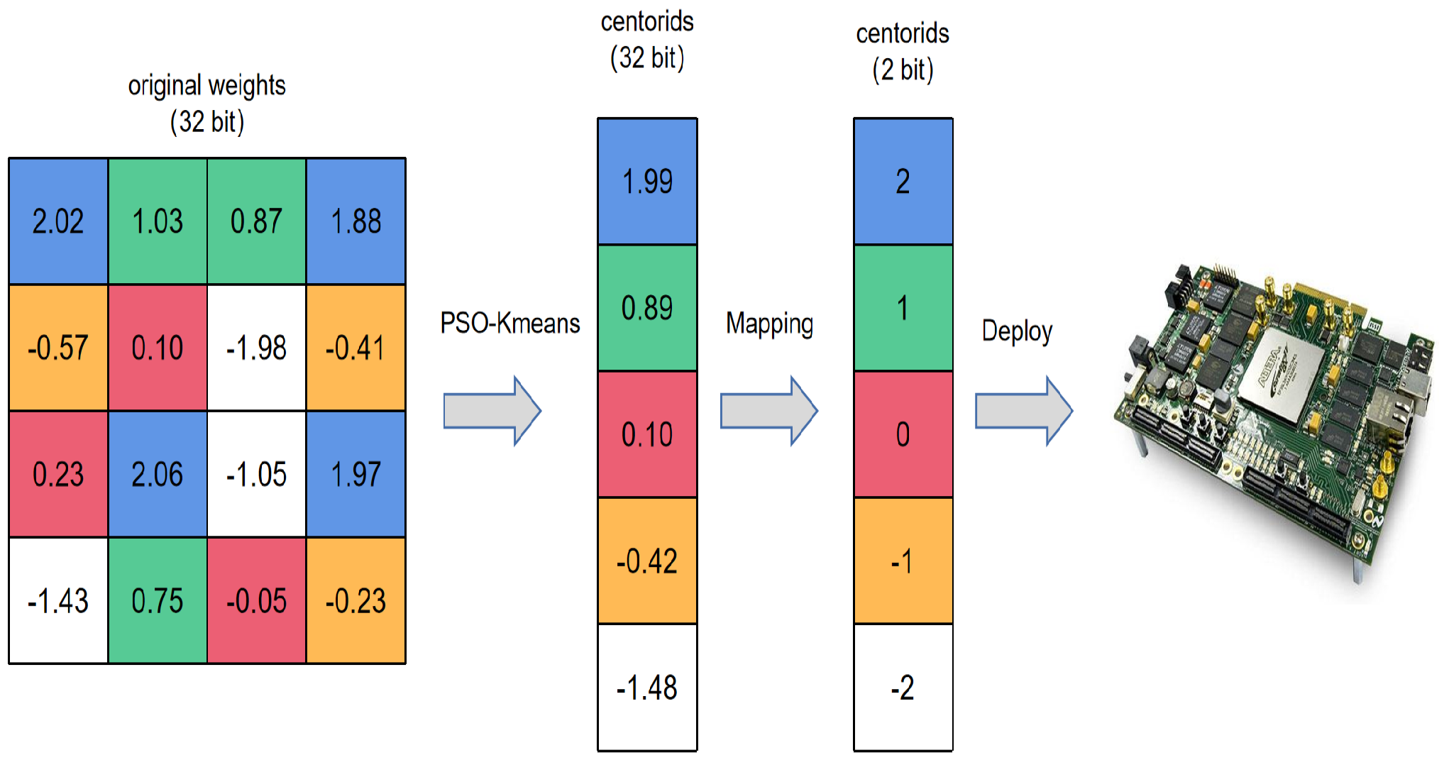
With PSO-K-means, each layer is divided into a certain number of groups determined by the quantization bit-width, and each group shares one centroid. To map cluster centroid into fixed-point numbers, a common practice is to use uniform partition (the process is shown in Figure 7). Through mapping, integer operations can be used to speed up the matrix operations of neural networks. The detail is shown in Algorithm 3.
For this paper, we define the following symbols:
- r denotes a real number;
- q denotes an n-bit integer.
Equation (8) shows the mapping of fixed-point q and floating-point r, where S and Z are the quantization parameters. Each layer of weights or activations shares a set of quantization parameters.
Note that the object to be quantified in this paper is the cluster centroids rather than the entire weight matrix. For the weight quantization, the core idea is to map the cluster centroids to a set of discrete, evenly spaced grid points which span the entire range. For example, with 8-bit quantization, the quantization range needs to be set to a symmetrical interval of [−127,127] instead of (−128,127].
| Algorithm 3 Mapping. |
| Input: weight matrix after clustering, Quantization bit-width n |
| Output: Result set |
|
4. Experiment
To evaluate the quantization method proposed in this paper, four popular CNN models for ImageNet classification are selected as benchmarks: ResNet-18 [33], ResNet-50 [33], DenseNet-121 [34], and Inception-v3 [35]. This paper tests on ImageNet ILSVRC-2012 [36] datasets. Their parameters are pre-trained on PyTorch [37]. The AGP in the Intel open-source Distiller [17] is used to prune the models. All the model pruning and quantization are implemented with CUDA 10.2 and PyTorch 1.4 frameworks for the Windows system on NVIDIA GeForce RTX 2080 Ti GPUs. The experiments in this paper will not quantize the first and last layer of the network because the first and last layer often requires higher accuracy [23].
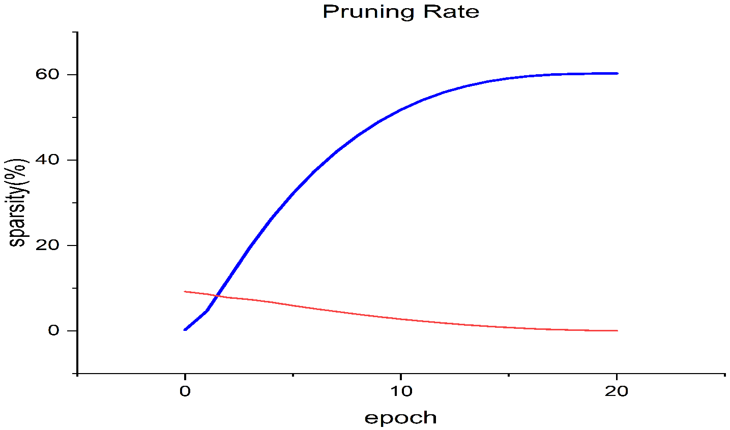
The models in the following experiments are all pruned models based on the AGP algorithm. Figure 8 is the pruning rate and sparsity curves of DenseNet-121 using the AGP algorithm. It is a pruner that controls the sparsity level growth by a mathematical formula and prunes the smallest magnitude weights to achieve a preset level of network sparsity [8]. Table 1 is the parameters used by the AGP algorithm, and Table 2 shows the top-1 and top-5 accuracies and sparsities of the models after pruning.
- Top-1 accuracy denotes the accuracy at which the top-ranked category matches the actual results.
- Top-5 accuracy denotes the accuracy at which the top-5 categories match the actual results.
- Total sparsity denotes the proportion of non-zero elements.
4.1. Accuracy Comparison between Linear Quantization and K-Means
In this section, this paper compares the impact of different clustering methods on the accuracy of the model. As mentioned above, linear quantization in this paper is treated as a combination of clustering and scaling. Its clustering function is based on uniform partition. Note that cluster centroids are not quantized. The number of cluster centroids is obtained by the bit-width.
According to the experimental results in Tabel Table 3, it can be found that the accuracy of uniform-partition and K-means at 6, 7, and 8 bits are almost the same. When the bit-width is further reduced, the difference in model accuracy is obvious. The experimental results show that the reason for the decrease in accuracy is consistent with the analysis in this paper.
The effect of clustering will directly affect the accuracy of the model. Because the distribution of weights is bell-shaped, the disadvantage is that the weights cannot be accurately distinguished by uniform partition when the bit-width is under 5 bits. By comparing the results of uniform partition and clustering, it can be concluded that if the weights can be accurately clustered, high accuracy can be maintained at low bit-widths.
4.2. Accuracy Comparison between Different Initialization Methods
To investigate how each quantization method affects performance, this paper considers three methods to determine the initial centroids of the cluster: random, uniform partition, and the PSO algorithm. The experimental results in Table 4 show that the particle swarm algorithm can effectively optimize the clustering results, and the accuracy is higher and more stable at the low bit-width than the methods using random and uniform partitions of the initial center of the cluster. According to the experimental results, we discover an interesting phenomenon, pruning will not cause the accuracy to decrease. On the contrary, when the bit-width is smaller than 5 bits, the accuracy of the model after pruning will be higher than the original model.
4.3. Accuracy Comparison between Existing Post Quantization Methods Based on Clipping
In Table 5 and Table 6, this paper compares the clipping-based method with our clustering-based method for two models, Resnet-50 and Inception-v3 on ImageNet, using the 4-bit precision. For ResNet-50, our methods increase the top-1 accuracy by 4.7% compared with the other post-quantization methods. For Inception-v3, our method increases the top-1 accuracy by 30.8% compared with the other post-quantization methods. This is strong evidence that the problem with linear quantization is that it cannot be reasonably clustered weights at low bit-widths.
5. Conclusions
This paper presents an optimized linear quantization method with a two-stage strategy including clustering and mapping. It improves low bit-width quantization without model retraining and can be easily applied to a common framework such as Distiller and Tensorflow-Lite. An interesting fact appears when evaluating how model pruning affects the model’s accuracy. Experimental results show that the accuracy of the model after pruning will be even higher than that of the original model when the quantization bit-width is less than 5 bits. Through unstructured pruning and quantization, the size of a DNN model can be reduced by at least 16×, which can effectively address the current extensive demands of edge applications for neural networks.
Different from the outlier clipping method proposed by previous quantization research works, this paper introduces a new thought by splitting the quantification process into two stages, clustering, and mapping. From the experiment results, it can be found that the accuracy loss is usually generated in the clustering stage. This paper adopts PSO-K-means to minimize the loss of accuracy. Compared with previous research clipping-based quantization methods, our two-stage quantization method achieves superior precision performance when using 4-bit precision. Thus, the proposed proposal of adding a clustering stage before the mapping stage can effectively maintain the distribution of weights, thereby reducing the loss of accuracy in the quantization process.
Future work can include more complex models such as RNNs (recurrent neural networks) and BERT for more in-depth research, as the current work is mainly focused on convolutional neural networks. Another effort for the future is to use other weight-sharing algorithms. In this article, we propose PSO-K-means as an algorithm for the clustering stage. In addition, there are many other weight-sharing algorithms that can be used.
Author Contributions
Conceptualization, W.Y.; Software, W.Y.; Formal analysis, W.Y.; Writing—original draft, W.Y.; Writing—review and editing, X.Z.; Supervision, X.Z. and W.T.; Project administration, X.Z. and W.T. All authors have read and agreed to the published version of the manuscript.
Funding
This work was funded in part by the Chinese Universities Industry-University-Research Innovation Foud under Grant No. 2020HYA02011, and in part by the Natural Science Foundation of Shandong Province under Grant No. ZR2019LZH002.
Data Availability Statement
Not applicable.
Acknowledgments
The authors gratefully appreciate the anonymous reviewers for their valuable comments.
Conflicts of Interest
All authors disclosed no relevant relationship.
References
- Lecun, Y.; Bengio, Y.; Hinton, G. Deep learning. Nature 2015, 521, 436. [Google Scholar] [CrossRef] [PubMed]
- Sallam, N.M. Speed control of three phase induction motor using neural network. IJCSIS 2018, 16, 16. [Google Scholar]
- Sallam, N.M.; Saleh, A.I.; Arafat Ali, H.; Abdelsalam, M.M. An Efficient Strategy for Blood Diseases Detection Based on Grey Wolf Optimization as Feature Selection and Machine Learning Techniques. Appl. Sci. 2022, 12, 10760. [Google Scholar] [CrossRef]
- Han, S.; Mao, H.; Dally, W.J. Deep Compression: Compressing Deep Neural Networks with Pruning, Trained Quantization and Huffman Coding. Fiber 2015, 56, 3–7. [Google Scholar]
- Xu, X.; Ding, Y.; Hu, S.X.; Niemier, M.; Cong, J.; Hu, Y.; Shi, Y. Scaling for edge inference of deep neural networks. Nat. Electron. 2018, 1, 216–222. [Google Scholar] [CrossRef]
- Reed, R.D. Pruning algorithms-a survey. IEEE Trans. Neural Netw. 1993, 4, 740–747. [Google Scholar] [CrossRef] [PubMed]
- Maarif, M.R.; Listyanda, R.F.; Kang, Y.-S.; Syafrudin, M. Artificial Neural Network Training Using Structural Learning with Forgetting for Parameter Analysis of Injection Molding Quality Prediction. Information 2022, 13, 488. [Google Scholar] [CrossRef]
- Zhu, M.; Gupta, S. To prune, or not to prune: Exploring the efficacy of pruning for model compression. arXiv 2017, arXiv:1710.01878. [Google Scholar]
- Vanhoucke, V.; Mao, M.Z. Improving the speed of neural networks on CPUs. In Proceedings of the Deep Learning and Unsupervised Feature Learning Workshop, NIPS 2011, Granada, Spain, 12–17 December 2011. [Google Scholar]
- Courbariaux, M.; Bengio, Y.; David, J.P. BinaryConnect: Training Deep Neural Networks with binary weights during propagations. In Proceedings of the International Conference on Neural Information Processing Systems, Montreal, QC, Canada, 7–12 December 2015. [Google Scholar]
- Leibe, B.; Matas, J.; Sebe, N.; Welling, M. XNOR-Net: ImageNet Classification Using Binary Convolutional Neural Networks. In Proceedings of the Computer Vision—ECCV 2016; Lecture Notes in Computer Science; Springer: Cham, Switzerland, 2016; Volume 9908, Chapter 32; pp. 525–542. [Google Scholar]
- Li, F.; Liu, B. Ternary Weight Networks. arXiv 2016, arXiv:1605.04711. [Google Scholar]
- Jacob, B.; Kligys, S.; Chen, B.; Zhu, M.; Tang, M.; Howard, A.; Adam, H.; Kalenichenko, D. Quantization and Training of Neural Networks for Efficient Integer-Arithmetic-Only Inference. In Proceedings of the IEEE Conference on Computer Vision and Pattern Recognition, Honolulu, HI, USA, 21–26 July 2017. [Google Scholar]
- Chang, S.E.; Li, Y.; Sun, M.; Shi, R.; So, H.K.-H.; Qian, X.; Wang, Y.; Lin, X. Mix and Match: A Novel FPGA-Centric Deep Neural Network Quantization Framework. In Proceedings of the 2021 IEEE International Symposium on High-Performance Computer Architecture (HPCA), Seoul, Republic of Korea, 27 February 27–3 March 2021. [Google Scholar]
- Migacz, S. 8-bit inference with TensorRT. In Proceedings of the GPU Technology Conference, San Jose, CA, USA, 8–11 May 2017. [Google Scholar]
- Han, S.; Pool, J.; Tran, J.; Dally, W. Learning both Weights and Connections for Efficient Neural Networks. In Advances in Neural Information Processing Systems; MIT Press: Cambridge, MA, USA, 2015. [Google Scholar]
- Zmora, N.; Jacob, G.; Elharar, B.; Zlotnik, L.; Novik, G.; Barad, H.; Chen, Y.; Muchsel, R.; Fan, T.J.; Chavez, R.; et al. NervanaSystems/Distillerv (V0.3.2). Zenodo. 2019. Available online: https://doi.org/10.5281/zenodo.3268730 (accessed on 1 January 2021).
- Miyashita, D.; Lee, E.H.; Murmann, B. Convolutional Neural Networks using Logarithmic Data Representation. arXiv 2016, arXiv:1603.01025. [Google Scholar]
- Chen, W.; Wilson, J.; Tyree, S.; Weinberger, K.; Chen, Y. Compressing Neural Networks with the Hashing Trick. In Proceedings of the International Conference on International Conference on Machine Learning, Lille, France, 6–11 July 2015. [Google Scholar]
- Wu, J.; Leng, C.; Wang, Y.; Hu, Q.; Cheng, J. Quantized Convolutional Neural Networks for Mobile Devices. In Proceedings of the 2016 IEEE Conference on Computer Vision and Pattern Recognition (CVPR), Las Vegas, NV, USA, 27–30 June 2016. [Google Scholar]
- Shin, S.; Hwang, K.; Sung, W. Fixed-point performance analysis of recurrent neural networks. In Proceedings of the 2016 IEEE International Conference on Acoustics, Speech and Signal Processing (ICASSP), Shanghai, China, 20–25 March 2016. [Google Scholar]
- Banner, R.; Nahshan, Y.; Soudry, D. Post training 4-bit quantization of convolutional networks for rapid-deployment. arXiv 2019, arXiv:1810.05723. [Google Scholar]
- Zhao, R. Improving Neural Network Quantization without Retraining using Outlier Channel Splitting. arXiv 2019, arXiv:1901.09504. [Google Scholar]
- Glover, F. Future paths for integer programming and links to artificial intelligence. Comput. Oper. Res. 1986, 13, 533–549. [Google Scholar] [CrossRef]
- Alorf, A. A survey of recently developed metaheuristics and their comparative analysis. Eng. Appl. Artif. Intell. 2023, 117, 105622. [Google Scholar] [CrossRef]
- Dorigo, M. Optimization, Learning and Natural Algorithms. Ph.D. Thesis, Politecnico di Milano, Milan, Italy, 1992. [Google Scholar]
- Kennedy, J.; Eberhart, R.C. Particle Swarm Optimization. In Proceedings of the IEEE International Joint Conference on Neural Networks, Perth, WA, Australia, 27 November–1 December 1995; Volume 4, pp. 1942–1948. [Google Scholar]
- Jain, M.; Singh, V.; Rani, A. A novel nature-inspired algorithm for optimization: Squirrel search algorithm. Swarm Evol. Comput. 2019, 44, 148–175. [Google Scholar] [CrossRef]
- Zhao, W.; Zhang, Z.; Wang, L. Manta ray foraging optimization: An effective bio-inspired optimizer for engineering applications. Eng. Appl. Artif. Intell. 2020, 87, 103300. [Google Scholar] [CrossRef]
- Omran, M.; Salman, A.; Engelbrecht, A.P. Image Classification using Particle Swarm Optimization. In Proceedings of the 4th Asia-Pacific Conference on Simulated Evolution and Learning, Singapore, 18–22 November 2002. [Google Scholar]
- Ballardini, A.L. A tutorial on Particle Swarm Optimization Clusterin. arXiv 2018, arXiv:1809.01942. [Google Scholar]
- Rousseeuw, P.J. Silhouettes: A graphical aid to the interpretation and validation of cluster analysis. J. Comput. Appl. Math. 1987, 20, 53–65. [Google Scholar] [CrossRef] [Green Version]
- He, K.; Zhang, X.; Ren, S.; Sun, J. Deep residual learning for image recognition. In Proceedings of the IEEE Conference on Computer Vision and Pattern Recognition (CVPR), Las Vegas, NV, USA, 27–30 June 2016; pp. 770–778. [Google Scholar]
- Huang, G.; Liu, Z.; Weinberger, K.Q.; van der Maaten, L. Densely connected convolutional networks. In Proceedings of the Conference on Computer Vision and Pattern Recognition (CVPR), Honolulu, HI, USA, 21–26 July 2017. [Google Scholar]
- Szegedy, C.; Liu, W.; Jia, Y.; Sermanet, P.; Reed, S.; Anguelov, D.; Erhan, D.; Vanhoucke, V.; Rabinovich, A. Going Deeper with Convolutions. In Proceedings of the Conference on Computer Vision and Pattern Recognition (CVPR), Boston, MA, USA, 7–12 June 2015. [Google Scholar]
- Deng, J.; Dong, W.; Socher, R.; Li, L.-J.; Li, K.; Li, F.-F. ImageNet: A Large-Scale Hierarchical Image Database. In Proceedings of the Conference on Computer Vision and Pattern Recognition (CVPR), Miami, FL, USA, 20–25 June 2009; pp. 248–255. [Google Scholar]
- Paszke, A.; Gross, S.; Chintala, S.; Chanan, G.; Yang, E.; DeVito, Z.; Lin, Z.; Desmaison, A.; Antiga, L.; Lerer, A. Automatic Differentiation in PyTorch. In Proceedings of the Advances in Neural Information Processing Systems Workshops (NIPS-W), Long Beach, CA, USA, 4–9 December 2017. [Google Scholar]
- Sung, W.; Shin, S.; Hwang, K. Resiliency of Deep Neural Networks under Quantization. arXiv 2015, arXiv:1511.06488. [Google Scholar]
Figure 1.
Synapses before and after pruning.

Figure 2.
Comparisons with existing quantization work based on clipping methods for ResNet-50, Inception-v3, and DenseNet-121 on ImageNet. (a) ResNet-50. (b) Inception-v3. (c) DenseNet-121.
Figure 2.
Comparisons with existing quantization work based on clipping methods for ResNet-50, Inception-v3, and DenseNet-121 on ImageNet. (a) ResNet-50. (b) Inception-v3. (c) DenseNet-121.

Figure 3.
In the effect of neural network sparsity on accuracy (based on Alexnet) [17]. It can be found that the convolutional layer is more sensitive to sparsity than the fully connected layer, and the depth of the convolutional layer will also affect the sensitivity. The deeper it is, the lower the sensitivity.

Figure 4.
Weight histogram for one of AlexNet’s convolutional and fully connected layers.

Figure 5.
Overview of two-stage quantization. It is composed of a clustering module and a mapping module. It takes as input a DNN model pretrained and pruned by some framework such as Pytorch.
Figure 5.
Overview of two-stage quantization. It is composed of a clustering module and a mapping module. It takes as input a DNN model pretrained and pruned by some framework such as Pytorch.

Figure 6.
Linear quantization loses inference accuracy when the bit-width is less than 5.

Figure 7.
The proposed DNN quantization framework with PSO-K-means and mapping.

Figure 8.
The pruning rate and sparsity curves of DenseNet-121 use the AGP algorithm.


Table 1.
The parameters of the AGP (automated gradual pruner) process.
| Network | Total Epochs | Initial Sparsity (%) | Final Sparsity (%) |
|---|---|---|---|
| ResNet-18 | 20 | 0 | 60 |
| ResNet-50 | 30 | 0 | 80 |
| Inception-V3 | 25 | 0 | 70 |
| Densenet-121 | 20 | 0 | 60 |
Table 2.
Top-1 and top-5 classification accuracies (%) on ImageNet2012 [33] validation dataset and the total sparsity (%) of network weights after pruning.
Table 2.
Top-1 and top-5 classification accuracies (%) on ImageNet2012 [33] validation dataset and the total sparsity (%) of network weights after pruning.
| Network | Top-1 (%) | Top-5 (%) | Total Sparsity (%) |
|---|---|---|---|
| ResNet-18 | 67.664 | 86.486 | 59.92 |
| ResNet-50 | 73.388 | 92.576 | 79.97 |
| Inception-V3 | 67.298 | 87.668 | 68.41 |
| Densenet-121 | 75.050 | 92.516 | 60.28 |
Table 3.
ImageNet top-1 accuracy with weight clustering—the float accuracy is displayed under the model name. Results include different cluster methods, uniform partition, and K-means.
Table 3.
ImageNet top-1 accuracy with weight clustering—the float accuracy is displayed under the model name. Results include different cluster methods, uniform partition, and K-means.
| Network | Bit-Width | Centroids | Linear | K-Means |
|---|---|---|---|---|
| ResNet-18 [33] (69.758) | 8 | 255 | 69.510 | 69.756 |
| 7 | 127 | 69.072 | 69.682 | |
| 6 | 63 | 67.290 | 69.494 | |
| 5 | 31 | 53.586 | 68.066 | |
| 4 | 15 | 1.028 | 61.466 | |
| ResNet-50 [33] (76.13) | 8 | 255 | 75.868 | 76.054 |
| 7 | 127 | 75.232 | 76.080 | |
| 6 | 63 | 72.532 | 75.382 | |
| 5 | 31 | 49.278 | 72.242 | |
| 4 | 15 | 0.234 | 67.736 | |
| DenseNet-121 [34] (74.433) | 8 | 255 | 74.266 | 74.380 |
| 7 | 127 | 73.458 | 74.260 | |
| 6 | 63 | 71.308 | 73.644 | |
| 5 | 31 | 56.260 | 72.738 | |
| 4 | 15 | 1.802 | 64.026 | |
| Inception-v3 [35] (69.538) | 8 | 255 | 69.968 | 69.478 |
| 7 | 127 | 67.942 | 69.288 | |
| 6 | 63 | 61.788 | 67.498 | |
| 5 | 31 | 12.892 | 63.414 | |
| 4 | 15 | 0.086 | 20.946 |
Table 4.
ImageNet top-1 validation accuracy with weight quantization—the float accuracy is displayed under the model name. Results include different initialization methods, random, uniform partition, and the PSO algorithm at each bit-width.
Table 4.
ImageNet top-1 validation accuracy with weight quantization—the float accuracy is displayed under the model name. Results include different initialization methods, random, uniform partition, and the PSO algorithm at each bit-width.
| Network | Bit-Width | Random (Before Pruning) | Random (After Pruning) | Uniform-Partition (After Pruning) | PSO (After Pruning) |
|---|---|---|---|---|---|
| ResNet-18 [33] (69.758) | 8 | 69.560 | 69.432 | 69.312 | 69.422 |
| 7 | 69.178 | 68.758 | 68.848 | 66.398 | |
| 6 | 67.906 | 68.540 | 67.660 | 68.114 | |
| 5 | 61.782 | 64.936 | 60.288 | 66.426 | |
| 4 | 49.134 | 55.328 | 50.720 | 59.594 | |
| ResNet-50 [33] (76.13) | 8 | 75.906 | 75.146 | 75.146 | 75.354 |
| 7 | 75.336 | 75.086 | 74.256 | 75.316 | |
| 6 | 75.280 | 74.620 | 74.182 | 75.050 | |
| 5 | 70.784 | 71.708 | 71.120 | 72.496 | |
| 4 | 60.736 | 65.208 | 64.630 | 67.622 | |
| DenseNet-121 [34] (74.433) | 8 | 74.138 | 74.530 | 74.140 | 74.064 |
| 7 | 73.876 | 73.138 | 73.330 | 74.006 | |
| 6 | 72.468 | 72.992 | 72.402 | 73.786 | |
| 5 | 70.856 | 70.712 | 68.130 | 72.392 | |
| 4 | 54.250 | 54.838 | 60.858 | 60.918 | |
| Inception-v3 [35] (69.538) | 8 | 68.382 | 66.916 | 66.656 | 67.220 |
| 7 | 68.048 | 66.43 | 67.070 | 67.364 | |
| 6 | 64.358 | 66.582 | 65.628 | 65.774 | |
| 5 | 56.420 | 57.200 | 55.514 | 60.958 | |
| 4 | 18.112 | 27.560 | 18.916 | 33.076 |
Table 5.
Comparisons with existing quantization work based on clipping methods for ResNet-50 on ImageNet, using the 4-bit precision. The quantization methods include linear, clip-linear, OCS-linear, and our two-stage quantization with PSO-K-means and mapping.
Table 5.
Comparisons with existing quantization work based on clipping methods for ResNet-50 on ImageNet, using the 4-bit precision. The quantization methods include linear, clip-linear, OCS-linear, and our two-stage quantization with PSO-K-means and mapping.
| Method | Approach | Bit-Width (Weight/Activation) | Top-1 (%) |
|---|---|---|---|
| Baseline | - | W32/A32 | 76.13 |
| none | Linear | W4/A4 | 0.1 |
| MSE [38] | Clip-Linear | W4/A4 | 45.0 |
| ACIQ [22] | Clip-Linear | W4/A4 | 33.2 |
| KL [15] | Clip-Linear | W4/A8 | 62.9 |
| OCS [23] | OCS-Linear | W4/A8 | 63.8 |
| PSO-K-means | Cluster-Map | W4/A4 | 67.622 |
Table 6.
Comparisons with existing quantization work based on clipping methods for Inception-v3 on ImageNet, using the 4-bit precision. The quantization methods include linear, clip-linear, OCS-linear, and our two-stage quantization with PSO-K-means and mapping.
Table 6.
Comparisons with existing quantization work based on clipping methods for Inception-v3 on ImageNet, using the 4-bit precision. The quantization methods include linear, clip-linear, OCS-linear, and our two-stage quantization with PSO-K-means and mapping.
| Method | Approach | Bit-Width (Weight/Activation) | Top-1 (%) |
|---|---|---|---|
| Baseline | - | W32/A32 | 69.538 |
| none | Linear | W4/A4 | 0.1 |
| MSE [38] | Clip-Linear | W4/A4 | 0.2 |
| ACIQ [22] | Clip-Linear | W4/A4 | 0.1 |
| KL [15] | Clip-Linear | W4/A8 | 1.6 |
| OCS [23] | OCS-Linear | W4/A8 | 2.3 |
| PSO-K-means | Cluster-Map | W4/A4 | 33.076 |
Disclaimer/Publisher’s Note: The statements, opinions and data contained in all publications are solely those of the individual author(s) and contributor(s) and not of MDPI and/or the editor(s). MDPI and/or the editor(s) disclaim responsibility for any injury to people or property resulting from any ideas, methods, instructions or products referred to in the content. |
© 2023 by the authors. Licensee MDPI, Basel, Switzerland. This article is an open access article distributed under the terms and conditions of the Creative Commons Attribution (CC BY) license (https://creativecommons.org/licenses/by/4.0/).
Share and Cite
MDPI and ACS Style
Yang, W.; Zhi, X.; Tong, W. Optimization of Linear Quantization for General and Effective Low Bit-Width Network Compression. Algorithms 2023, 16, 31. https://doi.org/10.3390/a16010031
AMA Style
Yang W, Zhi X, Tong W. Optimization of Linear Quantization for General and Effective Low Bit-Width Network Compression. Algorithms. 2023; 16(1):31. https://doi.org/10.3390/a16010031
Chicago/Turabian StyleYang, Wenxin, Xiaoli Zhi, and Weiqin Tong. 2023. "Optimization of Linear Quantization for General and Effective Low Bit-Width Network Compression" Algorithms 16, no. 1: 31. https://doi.org/10.3390/a16010031
Note that from the first issue of 2016, this journal uses article numbers instead of page numbers. See further details here.