
Sensor Placement with Two-Dimensional Equal Arc Length Non-Uniform Sampling for Underwater Terrain Deformation Monitoring


Abstract
:1. Introduction
1.1. Monitoring Methods for Underwater Terrain Deformation
1.2. Sensor Placement Schemes for Underwater Terrain Deformation
2. Two-Dimensional Non-Uniform Sampling Condition with Equal Arc Length
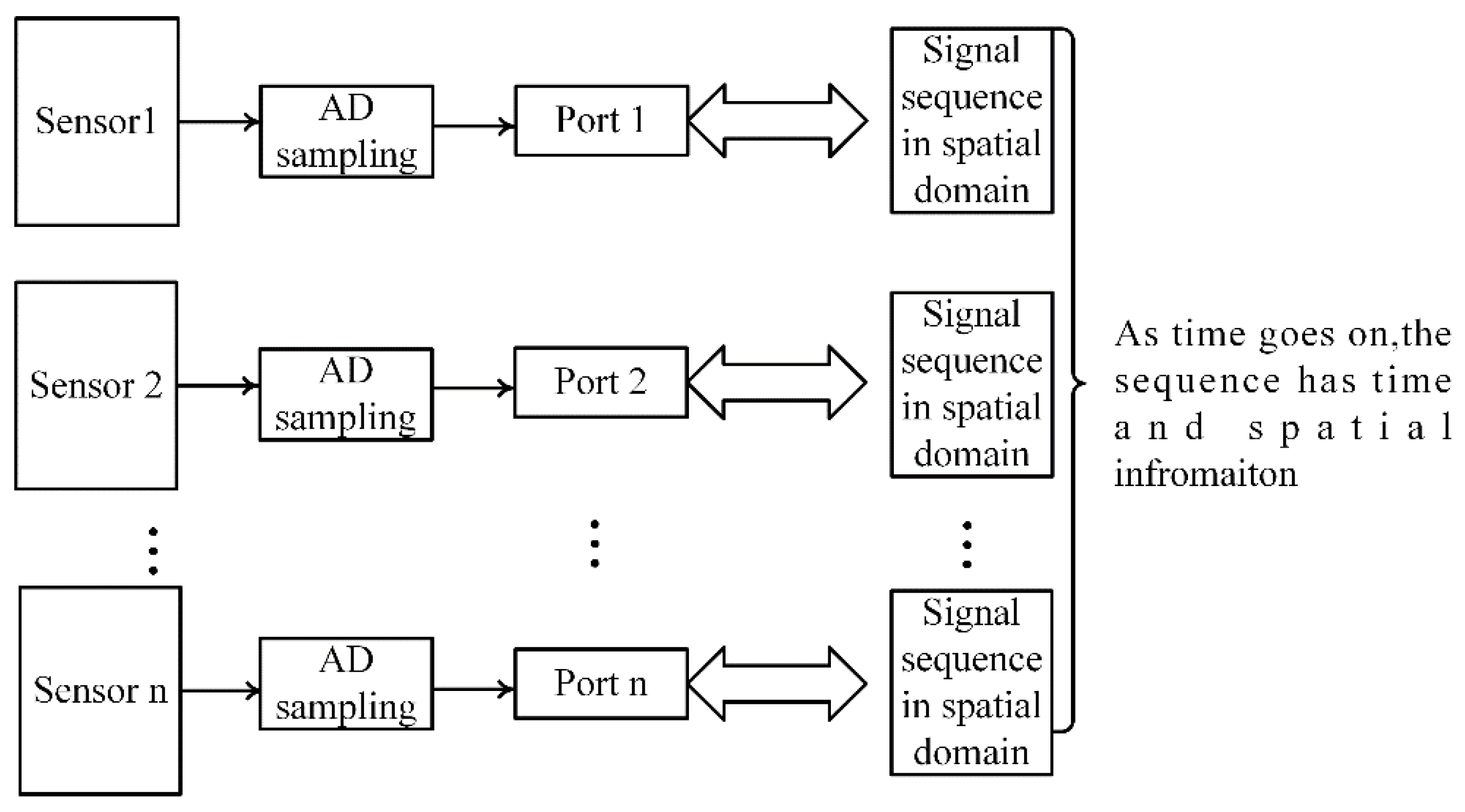
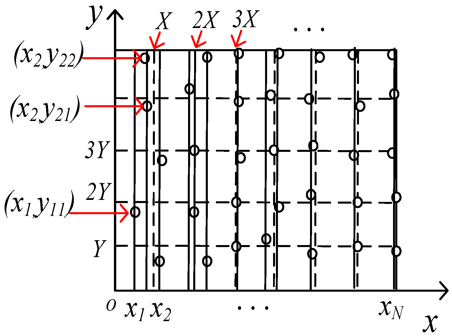
2.1. Mathematical Model of Two-Dimensional Uniform Sampling
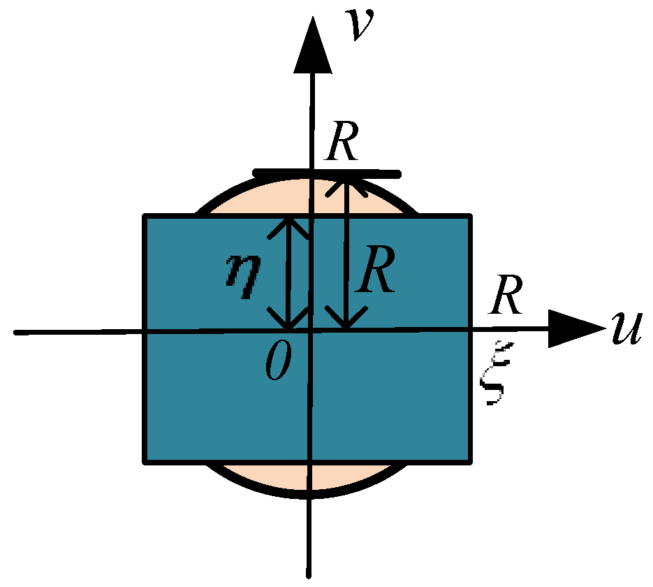
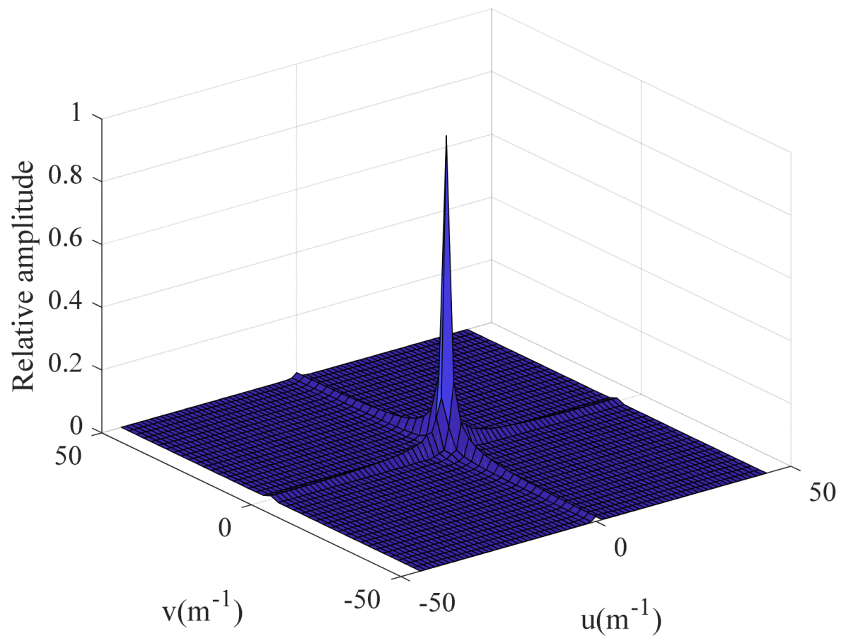
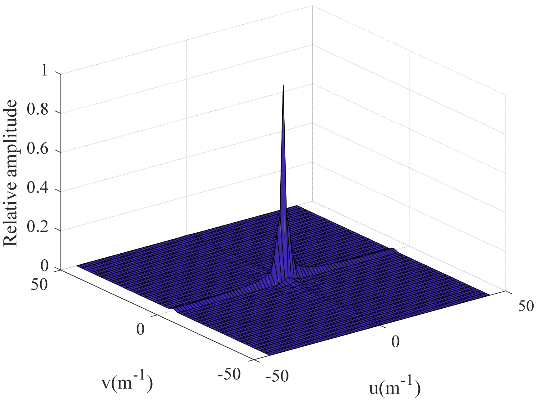
2.2. Two-Dimensional Non-Uniform Sampling Condition with Equal Arc Length
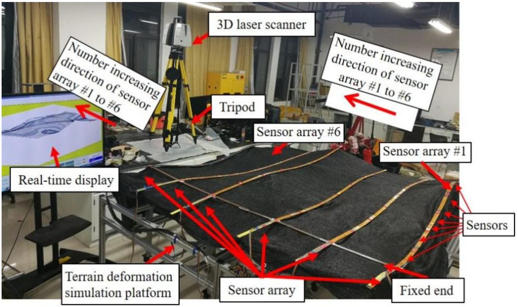
3. Terrain Deformation Simulation Experiment
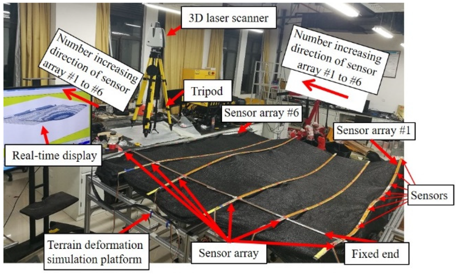
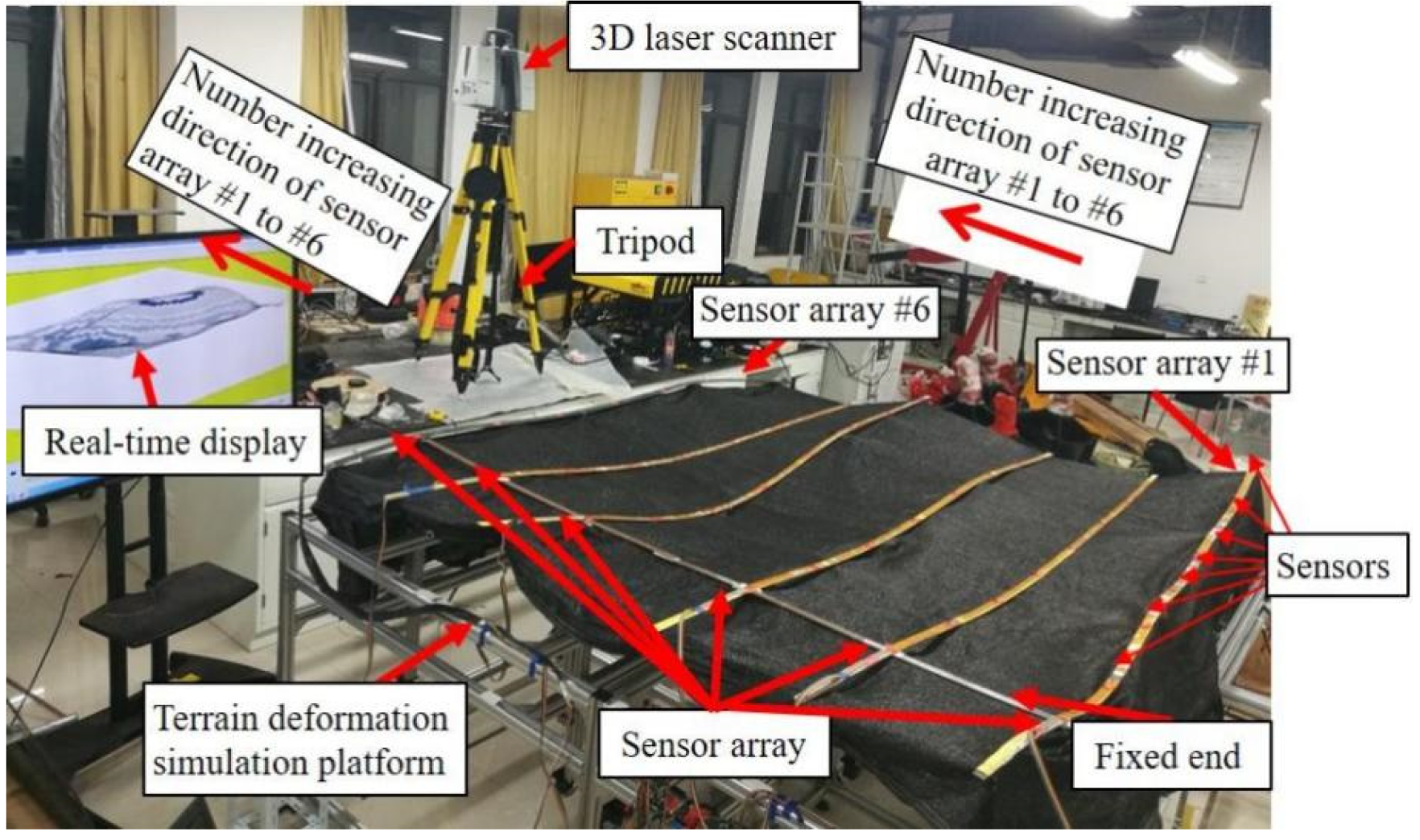
3.1. Experiment Design
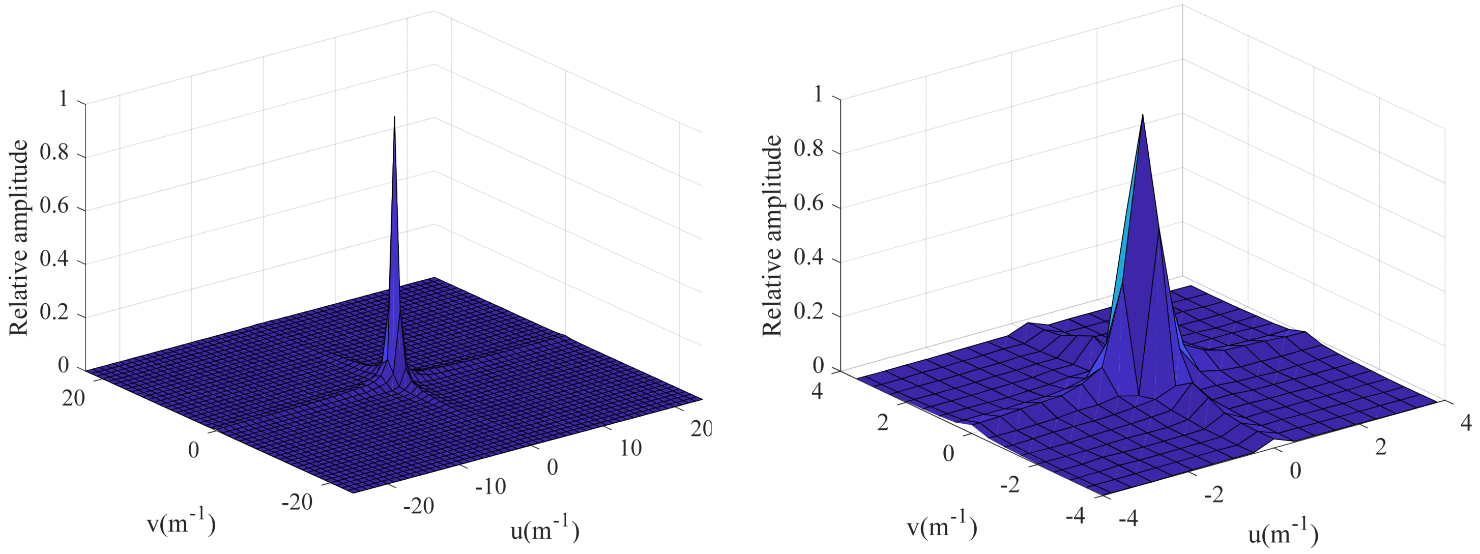
3.2. Experimental Results
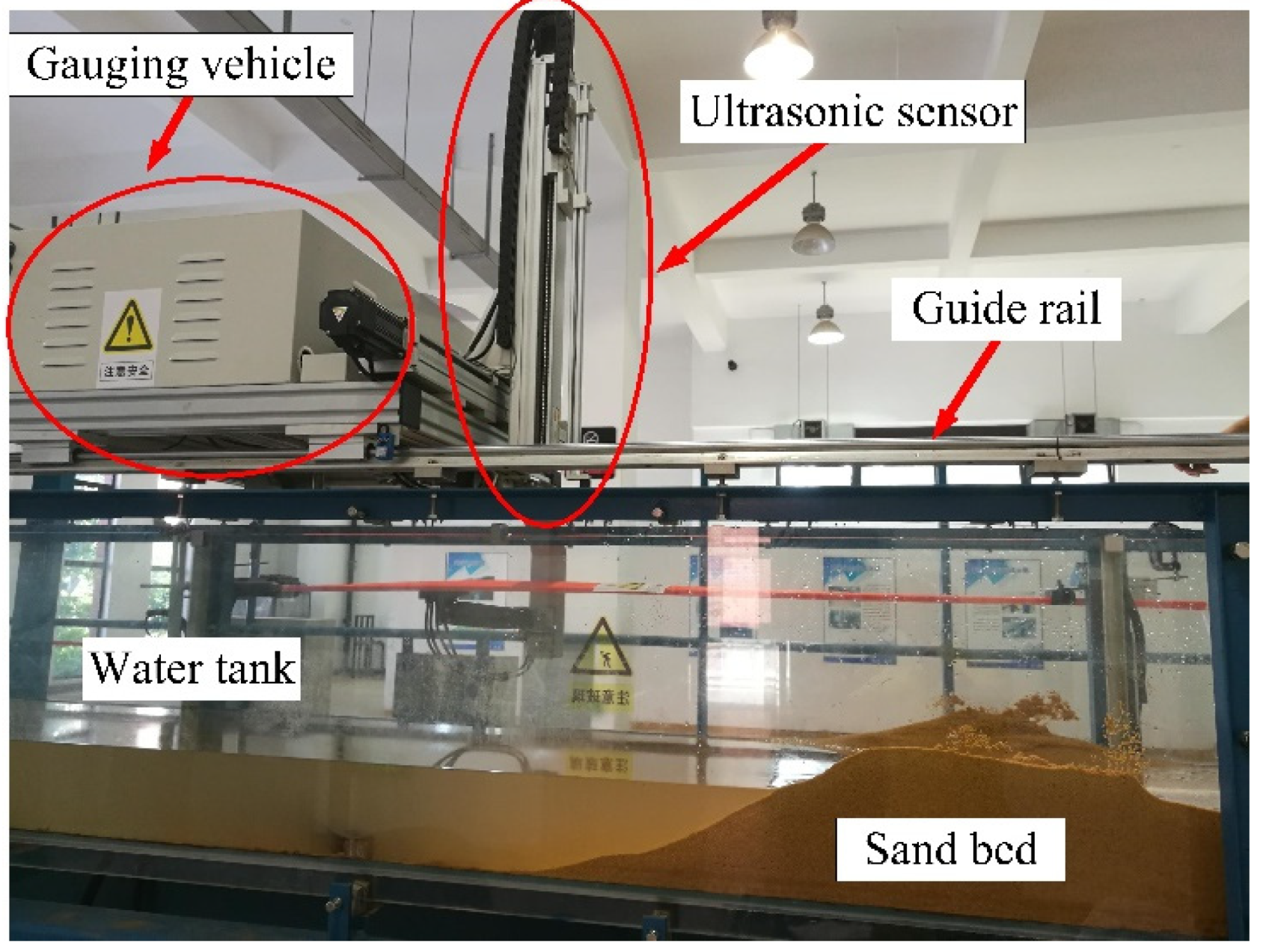
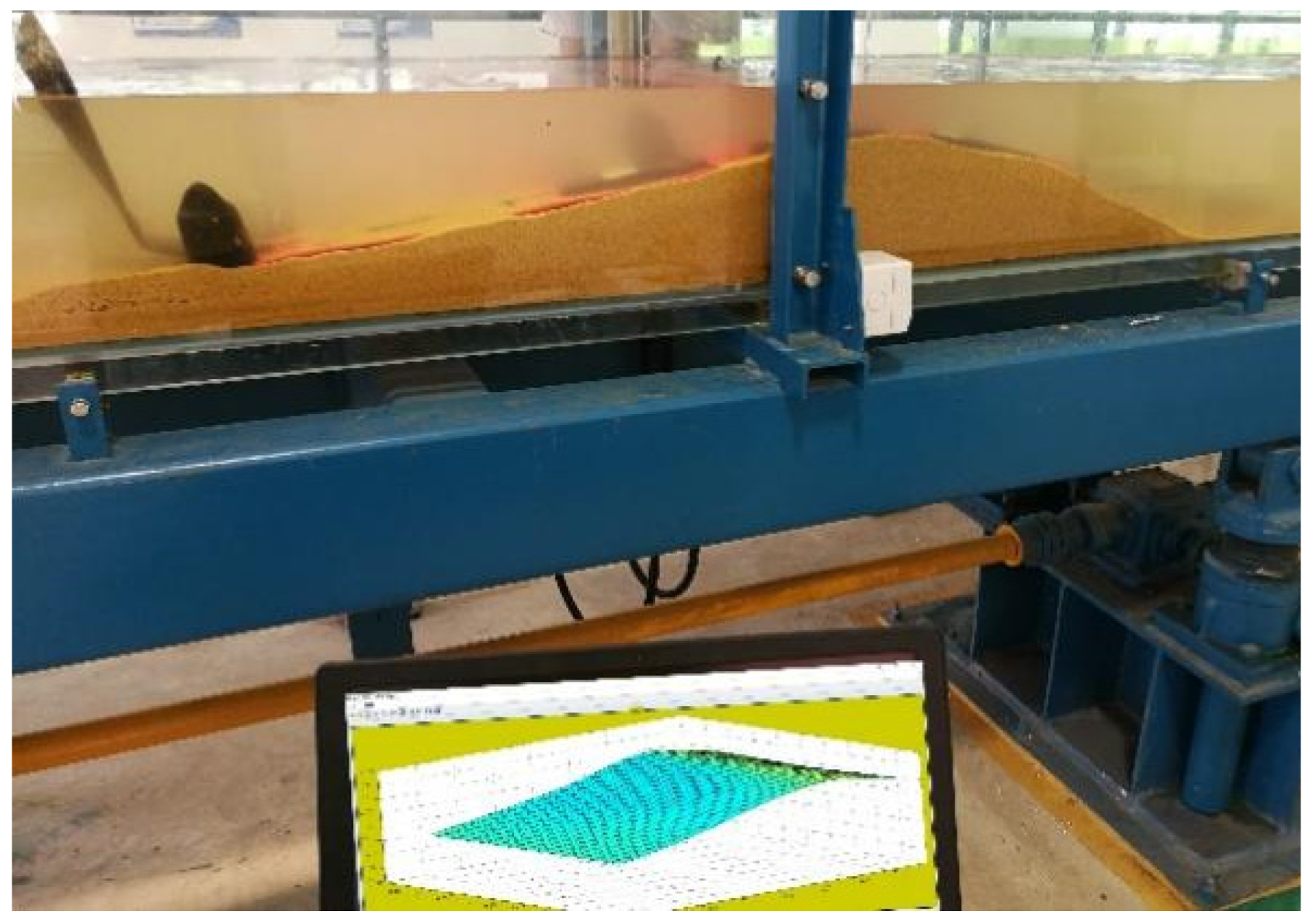
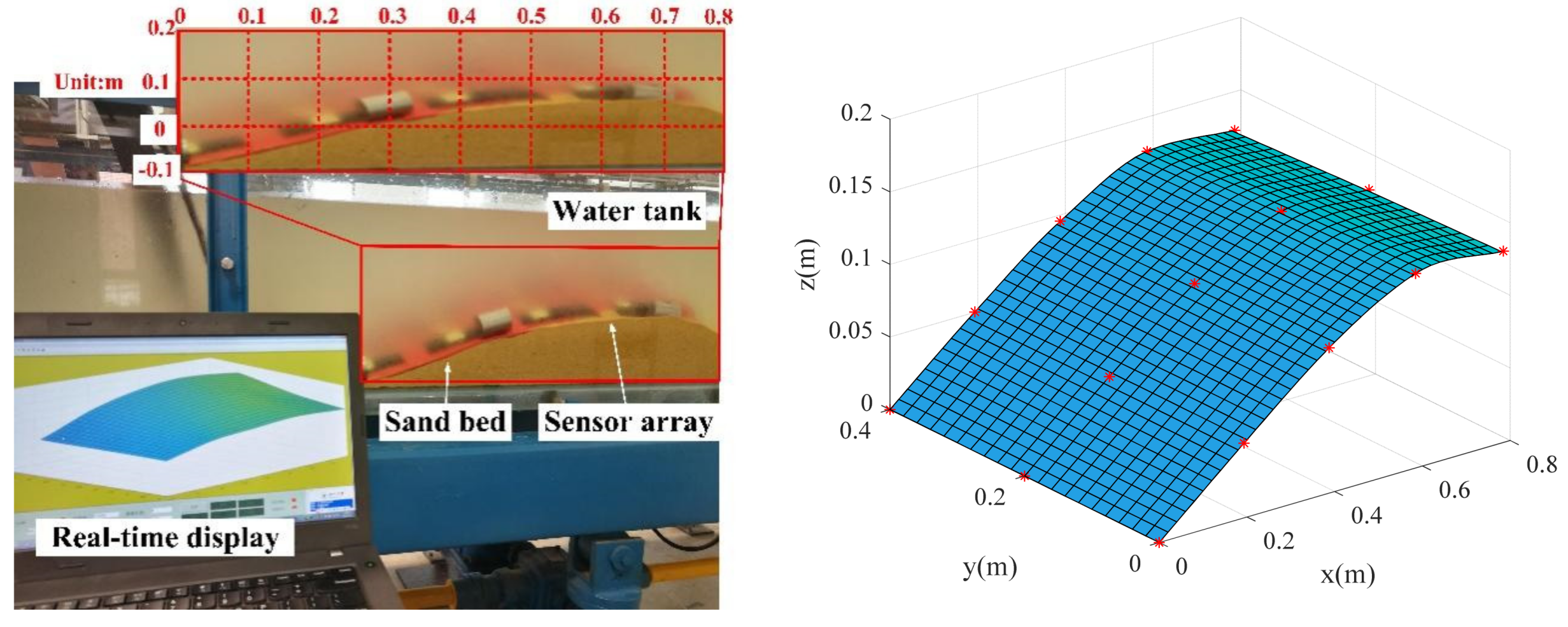
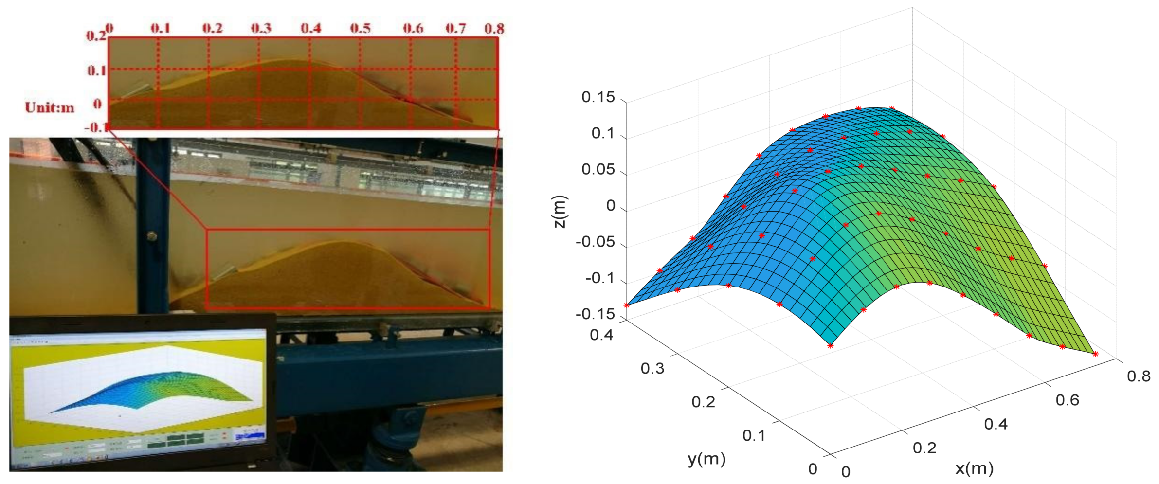
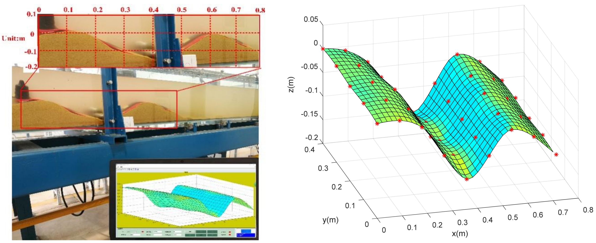
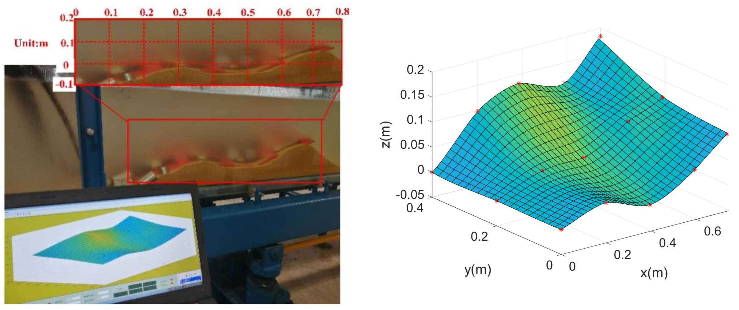
4. A Water Tank Experiment
4.1. Experiment Design
4.2. Experimental Results
5. Conclusions
Author Contributions
Funding
Institutional Review Board Statement
Informed Consent Statement
Data Availability Statement
Conflicts of Interest
References
- Wang, Z.; Jia, Y.; Liu, X.; Wang, D.; Shan, H.; Guo, L.; Wei, W. In situ observation of storm-wave-induced seabed deformation with a submarine landslide monitoring system. Bull. Eng. Geol. Environ. 2018, 77, 1091–1102. [Google Scholar] [CrossRef]
- Putti, S.P.; Satyam, N. Evaluation of Site Effects Using HVSR Microtremor Measurements in Vishakhapatnam (India). Earth Syst. Environ. 2020, 4, 439–454. [Google Scholar] [CrossRef]
- Shi, Y.H.; Liang, Q.Y.; Yang, J.P.; Yuan, Q.M.; Kong, L. Stability analysis of submarine slopes in the area of the test production of gas hydrate in the south china sea. China Geol. 2019, 2, 276–286. [Google Scholar] [CrossRef]
- Vanneste, M.; Sultan, N.; Garziglia, S.; Forsberg, C.F.; L’Heureux, J.S. Seafloor instabilities and sediment deformation processes: The need for integrated, multi-disciplinary investigations. Mar. Geol. 2014, 352, 183–214. [Google Scholar] [CrossRef] [Green Version]
- Amiri-Simkooei, A.R.; Snellen, M.; Simons, D.G. Principal component analysis of single-beam echo-sounder signal features for seafloor classification. IEEE J. Ocean. Eng. 2011, 36, 259–272. [Google Scholar] [CrossRef]
- Hefner, B.T. Characterization of seafloor roughness to support modeling of midfrequency reverberation. IEEE J. Ocean. Eng. 2017, 42, 1110–1124. [Google Scholar] [CrossRef]
- Calvert, J.; Strong, J.A.; Service, M.; McGonigle, C.; Quinn, R. An evaluation of supervised and unsupervised classification techniques for marine benthic habitat mapping using multibeam echosounder data. ICES J. Mar. Sci. 2015, 72, 1498–1513. [Google Scholar] [CrossRef] [Green Version]
- Holler, P.; Markert, E.; Bartholom, A.; Capperucci, R.; Reimers, H.C. Tools to evaluate seafloor integrity: Comparison of multi-device acoustic seafloor classifications for benthic macrofauna-driven patterns in the german bight, southern north sea. Geo-Mar. Lett. 2016, 37, 1–17. [Google Scholar] [CrossRef]
- Lamarche, G.; Lurton, X. Recommendations for improved and coherent acquisition and processing of backscatter data from seafloor-mapping sonars. Mar. Geophys. Res. 2018, 39, 5–22. [Google Scholar] [CrossRef] [Green Version]
- Zhu, H.H.; Shi, B.; Yan, J.F.; Zhang, J.; Wang, B.J. Fiber bragg grating-based performance monitoring of a slope model subjected to seepage. Smart Mater. Struct. 2014, 23, 1–12. [Google Scholar] [CrossRef]
- Moe, A.; Aminossadati, S.M.; Kizil, M.S.; Rakić, A.D. Recent developments in fibre optic shape sensing. Measurement 2018, 128, 119–137. [Google Scholar]
- Hauswirth, D.; Puzrin, A.M.; Carrera, A.; Standing, J.R.; Wan, M.S.P. Use of fibre-optic sensors for simple assessment of ground surface displacements during tunneling. Geothchnique 2014, 64, 837–842. [Google Scholar] [CrossRef]
- Zhang, Y.; Tang, H.; Li, C.; Lu, G.; Cai, Y.; Zhang, J.; Tan, F. Design and testing of a flexible inclinometer probe for model tests of landslide deep displacement measurement. Sensors 2018, 18, 224. [Google Scholar] [CrossRef] [PubMed] [Green Version]
- Xu, C.; Chen, J.; Zhu, H.; Liu, H.; Lin, Y. Experimental research on seafloor mapping and vertical deformation monitoring for gas hydrate zone using nine-axis MEMS sensor tapes. IEEE J. Ocean. Eng. 2018, 44, 1090–1101. [Google Scholar] [CrossRef]
- Xu, C.; Chen, J.; Ge, Y.; Ren, Z.; Cao, C.; Zhu, H.; Huang, Y.; Wang, H.; Wang, W. Monitoring the vertical changes of a tidal flat using a mems accelerometer array. Appl. Ocean. Res. 2020, 101, 102186. [Google Scholar] [CrossRef]
- Leal-Junior, A.G.; Frizera-Neto, A.; Pontes, M.J.; Botelho, T.R. Hysteresis compensation technique applied to polymer optical fiber curvature sensor for lower limb exoskeletons. Meas. Sci. Technol. 2017, 28, 125103. [Google Scholar] [CrossRef]
- Leal-Junior, A.G.; Anselmo, F.; Avellar, L.M.; Pontes, M.J. Design considerations, analysis, and application of a low-cost, fully portable, wearable polymer optical fiber curvature sensor. Appl. Opt. 2018, 57, 6927–6936. [Google Scholar] [CrossRef]
- Gong, H.; Xiao, Y.; Kai, N.; Zhao, C.L.; Dong, X. An optical fiber curvature sensor based on two peanut-shape structures modal interferometer. IEEE Photonic Technol. Lett. 2013, 26, 22–24. [Google Scholar] [CrossRef]
- De Kim, T.; Youn, B.D.; Oh, H. Development of a stochastic effective independence (sefi) method for optimal sensor placement under uncertainty. Mech. Syst. Signal Process. 2018, 111, 615–627. [Google Scholar] [CrossRef]
- Kang, L.; Ren-Jun, Y.; Guedes, S.C. Optimal sensor placement and assessment for modal identification. Ocean Eng. 2018, 165, 209–220. [Google Scholar]
- Ameyaw, D.A.; Rothe, S.; Söffker, D. Fault diagnosis using probability of detection (pod)-based sensor/information fusion for vibration-based analysis of elastic structures. PAMM 2018, 18, 1–2. [Google Scholar] [CrossRef]
- Tong, K.H.; Bakhary, N.; Kueh, A.; Yassin, A. Optimal sensor placement for mode shapes using improved simulated annealing. Smart Struct. Syst. 2014, 13, 389–406. [Google Scholar] [CrossRef]
- Gomes, G.F.; Almeida, F.D.; Alexandrino, P.L. A multiobjective sensor placement optimization for SHM systems considering fisher information matrix and mode shape interpolation. Eng. Comput.-Ger. 2019, 35, 519–535. [Google Scholar] [CrossRef]
- Downey, A.; Hu, C.; Laflamme, S. Optimal sensor placement within a hybrid dense sensor network using an adaptive genetic algorithm with learning gene pool. Struct. Health Monit. 2017, 17, 450–460. [Google Scholar] [CrossRef] [Green Version]
- Marks, R.; Clarke, A.; Featherston, C.A.; Pullin, R. Optimization of acousto-ultrasonic sensor networks using genetic algorithms based on experimental and numerical data sets. Int. J. Distrib. Sens. Netw. 2017, 13. [Google Scholar] [CrossRef]
- Huang, Y.; Ludwig, S.A.; Deng, F. Sensor optimization using a genetic algorithm for structural health monitoring in harsh environments. J. Civ. Struct. Health Monit. 2016, 6, 509–519. [Google Scholar] [CrossRef]
- Long, D.G.; Franz, R. Band-Limited signal reconstruction from irregular samples with variable apertures. IEEE Trans. Geosci. Remote 2016, 54, 2424–2436. [Google Scholar] [CrossRef]
- Hu, Y.; Fan, Y.; Wei, Y.; Wang, Y.; Liang, Q. Subspace-based continuous-time identification of fractional order systems from non-uniformly sampled data. Int. J. Sys. Sci. 2016, 47, 122–134. [Google Scholar] [CrossRef]
- Souglo, K.E. Non-uniform distributions of initial porosity in metallic materials affect the growth rate of necking instabilities in flat tensile samples subjected to dynamic loading. Mech. Res. Commun. 2018, 91, 87–92. [Google Scholar]
- Zhao, S.; Wang, R.; Deng, Y.; Zhang, Z.; Li, N.; Guo, L.; Wang, W. Modifications on multichannel reconstruction algorithm for SAR processing based on periodic nonuniform sampling theory and nonuniform fast fourier transform. IEEE J. Sel. Top. Appl. Earth Obs. Remote. Sens. 2015, 8, 4998–5006. [Google Scholar] [CrossRef]
- Marvasti, F. Nonuniform Sampling: Theory and Practice; Kluwer Academic: Dordrecht, The Netherlands, 2001. [Google Scholar]
- Haykin, S.; Barry, V.V. Signals and Systems, 2nd ed.; Wiley: Hoboken, NJ, USA, 2003. [Google Scholar]


| Shape #1-1 | Shape #1-2 | Shape #1-3 | |
|---|---|---|---|
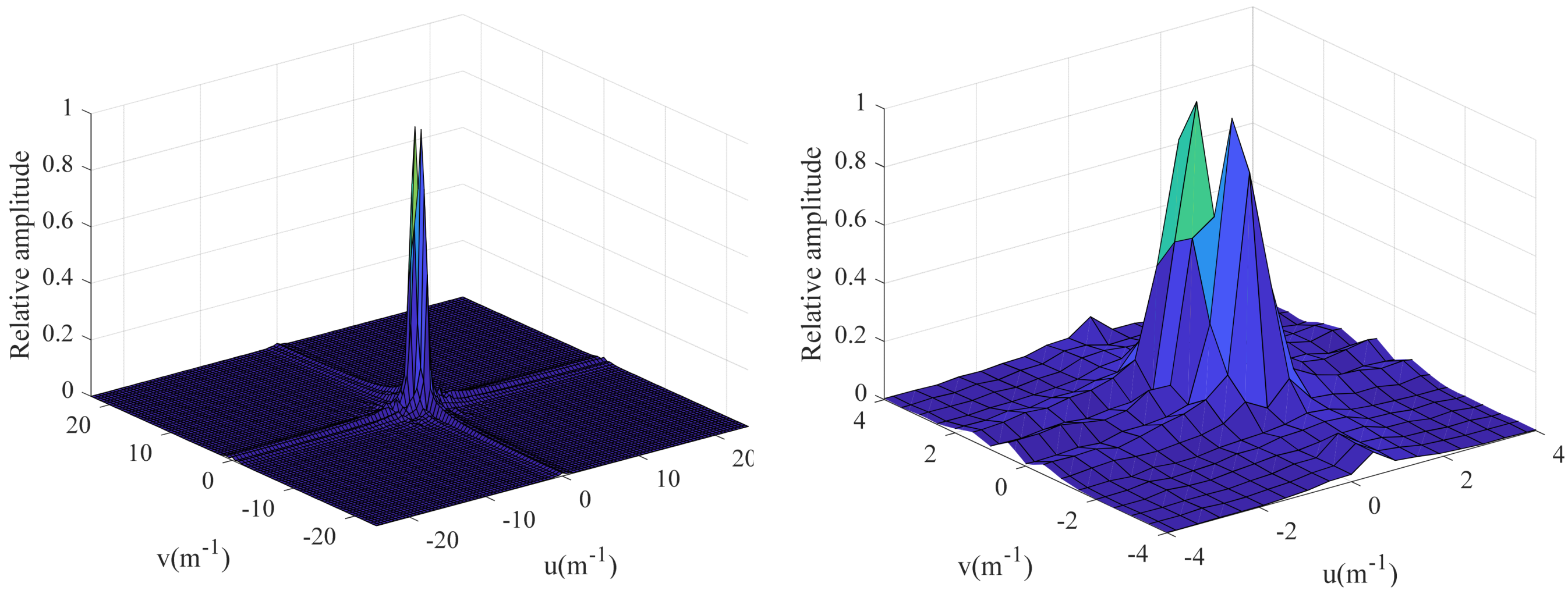
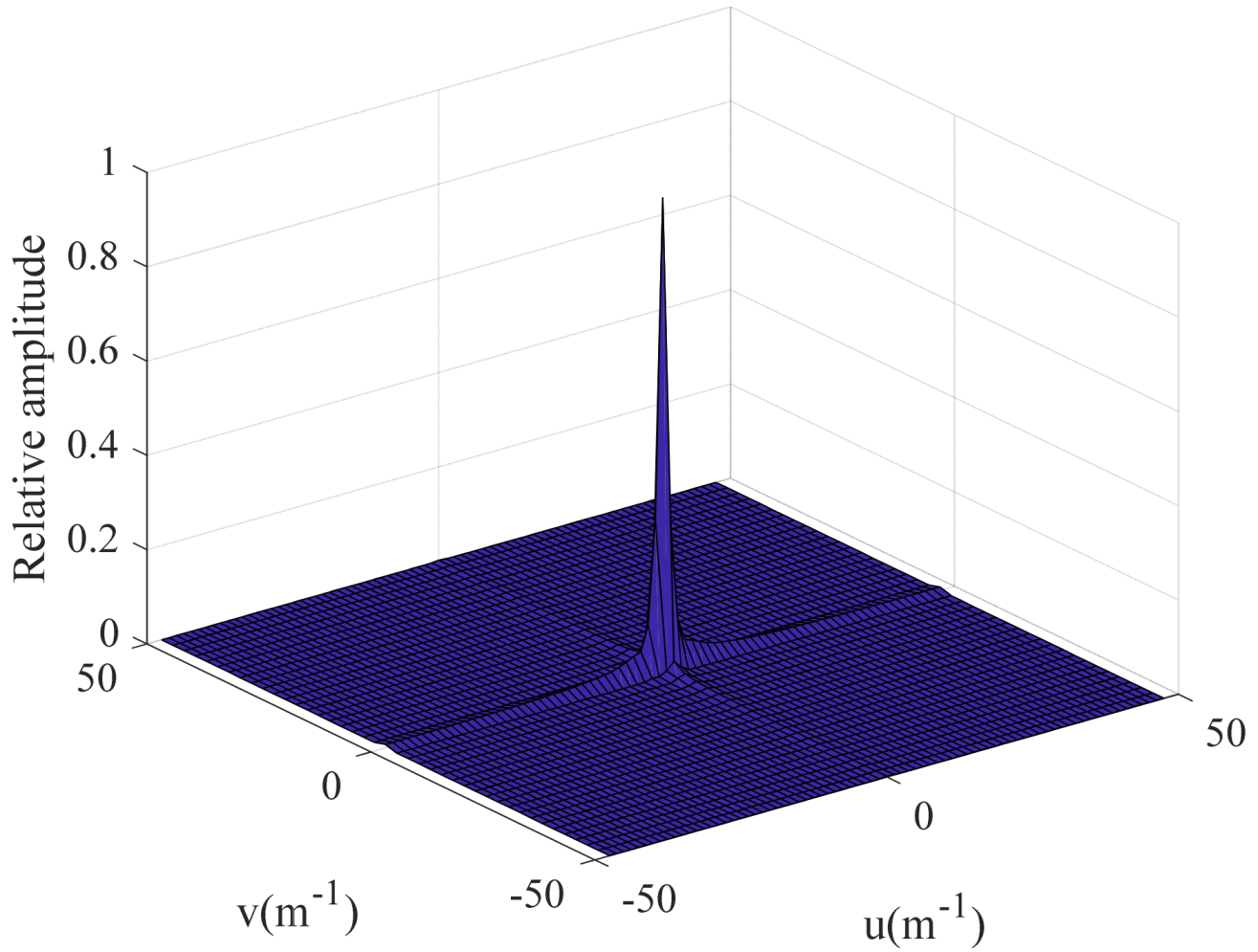
| Highest frequency (u, v) (m−1) | (0.94, 1.10) | (1.41, 1.10) | (0.94, 1.10) |
| Shape #1-1 | Shape #1-2 | Shape #1-3 | |
|---|---|---|---|
| Mean absolute error (cm) | 1.12 | 0.97 | 1.09 |
| MRE (%) | 6.47 | 6.87 | 5.09 |
| RRMSE (%) | 6.01 | 5.53 | 4.43 |
| Shape #2-1 | Shape #2-2 | Shape #2-3 | |
|---|---|---|---|
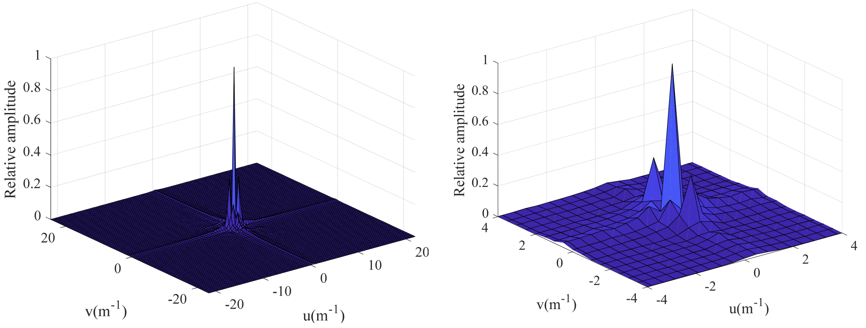
| Highest frequency (u, v) (m−1) | (1.25, 2.5) | (2.5, 2.5) | (1.25, 2.5) |
| Shape #2-1 | Shape #2-2 | Shape #2-3 | Shape #2-4 | Shape #2-5 | |
|---|---|---|---|---|---|
| MRE (%) | 3.29 | 5.62 | 3.36 | 5.71 | 3.48 |
| RRMSE (%) | 3.52 | 5.89 | 3.45 | 6.73 | 3.02 |
Publisher’s Note: MDPI stays neutral with regard to jurisdictional claims in published maps and institutional affiliations. |
© 2021 by the authors. Licensee MDPI, Basel, Switzerland. This article is an open access article distributed under the terms and conditions of the Creative Commons Attribution (CC BY) license (https://creativecommons.org/licenses/by/4.0/).
Share and Cite
Xu, C.; Hu, J.; Chen, J.; Ge, Y.; Liang, R. Sensor Placement with Two-Dimensional Equal Arc Length Non-Uniform Sampling for Underwater Terrain Deformation Monitoring. J. Mar. Sci. Eng. 2021, 9, 954. https://doi.org/10.3390/jmse9090954
Xu C, Hu J, Chen J, Ge Y, Liang R. Sensor Placement with Two-Dimensional Equal Arc Length Non-Uniform Sampling for Underwater Terrain Deformation Monitoring. Journal of Marine Science and Engineering. 2021; 9(9):954. https://doi.org/10.3390/jmse9090954
Chicago/Turabian StyleXu, Chunying, Junwei Hu, Jiawang Chen, Yongqiang Ge, and Ruixin Liang. 2021. "Sensor Placement with Two-Dimensional Equal Arc Length Non-Uniform Sampling for Underwater Terrain Deformation Monitoring" Journal of Marine Science and Engineering 9, no. 9: 954. https://doi.org/10.3390/jmse9090954