Artificial Bee Colony Programming Descriptor for Multi-Class Texture Classification


Department of Computer Engineering Erciyes University, Engineering Faculty Computer Engineering, Kayseri 38000, Turkey
*
Author to whom correspondence should be addressed.
Appl. Sci. 2019, 9(9), 1930; https://doi.org/10.3390/app9091930
Submission received: 4 April 2019
/
Revised: 29 April 2019
/
Accepted: 8 May 2019
/
Published: 10 May 2019
(This article belongs to the Special Issue Machine Learning and Compressed Sensing in Image Reconstruction)
Abstract
:Featured Application
Texture classification aims to identify textures using few samples. Local Binary Pattern (LBP) and GP-descriptor are most used texture classification algorithms. Artificial Bee Colony Programming-Descriptor (ABCP-Descriptor) evaluates samples to extract mathematical models. Comparative results show that proposed ABCP-Descriptor is a successful texture classification method.
Abstract
Texture classification is one of the machine learning methods that attempts to classify textures by evaluating samples. Extracting related features from the samples is necessary to successfully classify textures. It is a very difficult task to extract successful models in the texture classification problem. The Artificial Bee Colony (ABC) algorithm is one of the most popular evolutionary algorithms inspired by the search behavior of honey bees. Artificial Bee Colony Programming (ABCP) is a recently introduced high-level automatic programming method for a Symbolic Regression (SR) problem based on the ABC algorithm. ABCP has applied in several fields to solve different problems up to date. In this paper, the Artificial Bee Colony Programming Descriptor (ABCP-Descriptor) is proposed to classify multi-class textures. The models of the descriptor are obtained with windows sliding on the textures. Each sample in the texture dataset is defined instance. For the classification of each texture, only two random selected instances are used in the training phase. The performance of the descriptor is compared standard Local Binary Pattern (LBP) and Genetic Programming-Descriptor (GP-descriptor) in two commonly used texture datasets. When the results are evaluated, the proposed method is found to be a useful method in image processing and has good performance compared to LBP and GP-descriptor.
1. Introduction
The image descriptor provides information about the image by extracting / determining features such as shape or color. Image descriptors have two different types: dense / sparse. Dense descriptors are the approaches that extract features from the image in a pixel-by-pixel. One of the most common dense descriptors is the Local Binary Pattern (LBP). Scale Invariant Feature Transform (SIFT) and Speeded up Robust Features (SURF) are examples of instances in which sparse descriptors evaluate each pixel in the image and extract the models [1].
Automatic programming is the process which the machine generates program code automatically [2]. GP, the most well-known automatic programming method, was developed by Koza [3]. GP is an extension of the Genetic Algorithm (GA) and the basic steps for the GP algorithm are similar to the GA steps. ABCP is the recently proposed automatic programming method based on Artificial Bee Colony (ABC) algorithm [4]. In this paper, the ABCP image descriptor was first proposed and the success of the extracted models in the texture classification problem was evaluated.
In recent years, automatic programming methods have been used more frequently in image processing problems. Tackett [5] used GP to classify feature vectors derived from images into categories. A domain adaptive learning method based on Multi-Objective Genetic Programming (MOGP) was proposed to automatically generate field-adaptive global property descriptors for image classification in [6]. GP was suggested for feature detection in [7]. The method separated the image into the sub-regions, extracted the Speeded up Robust Features (SURF) points and achieved successful classification results using the Support Vector Machine (SVM) classifier. Iqbal et al. proposed an image classification method using transfer learning and GP [8]. The GP trees are extracted by the fragments of the transfer learning improved classification performance producing more useful initial population. In [9], they introduced new GP method that automatically differentiated the regions in the image and sorted them out by extracting Histograms of Oriented Gradients (HOG). All stages of the method were optimized with wide search space. Al-Sahaf et al. proposed a Two-Tier GP (Two-Tier GP, Two-Tier GP-line, and Two-Tier GP-mix) with three different variations [10]. Instead of using them as input values, they defined special functions that can convert line pixel values into a single numeric value, and in the other tier, classification was made by using the outputs of special functions. Two Tier GP-mix was considered the most successful method because of the flexibility of the window range.
Comparative studies of ABC with Particle Swarm Optimization, GA and other evolutionary computational algorithms have shown that ABC has better performance in terms of achieving local and global optimum results in engineering problems [11]. ABC is an algorithm that is successfully applied in image processing, especially in image clustering [12], image registration [13], pattern recognition [14], image segmentation [15,16,17,18,19], and image classification [20]. ABC algorithm was used in the diagnosis of computed tomography images in [20]. The images are classified with k Nearest Neighbor (k-NN) and SVM classifiers by selecting features with ABC. The ABC-SVM hybrid is highly successful. The ABCP algorithm has been proposed as an ABC-based method that improves functions on symbolic regression [4]. This is the first paper that observes the performance of the ABCP algorithm in texture classification and extracts mathematical models.
Nowadays, due to its simplicity of calculation and its robustness against light changes, LBP-based descriptors have been extensively researched due to its importance in various fields such as image classification problem, pattern recognition and computer vision [21,22,23,24,25]. [21] was proposed a GP-based LBP image descriptor using one instance per class. The method was shown to be more successful against five different methods with / without GP-based. Ojala et al. presented a uniform LBP (uniform LBP) approach in rotation-sensitive, simple and gray-scale variances [22]. Sinha et al. proposed the Wigner-based LBP identifier (WLBP, Wigner-Based Local Binary Patterns), which uses the Wigner distribution together with LBP [23]. In experiments using different classifiers, the method performed better than conventional LBP. [24] was presented a two-part Feature Based Local Binary Pattern (FB-LBP) approach. In the first part, traditional LBP is used, while in the other part the mean and variance of the magnitude vector is used. Liu et al. proposed a novel local texture descriptor, generalizing the well-known LBP approach. Four LBP-like descriptors, two local intensity-based Central Intensity LBP (CI-LBP) and Neighbors Intensity LBP (NI-LBP), and two local difference-based descriptors Radial Difference LBP (RD-LBP) and Angular Difference LBP(AD-LBP), were presented to extract complementary texture information of local spatial patterns [1]. The descriptors had the same structure as the standard LBP and not require training and parameter adjustment. In the study conducted in three different texture, the descriptors showed better performance in gray-scale and rotation-sensitive pattern classification compared to traditional LBP.
A plethora of neural networks have been presented image processing [25,26,27]. Zhang et al. introduced a two-stage approach to the use of pixel based neural networks trained by back propagation and GA [26]. The network is trained on samples, which cut out of from large pictures. In the first stage, weights of networks are adjusted GA and in the second stage they tested the method on three object detection problems. The results show that the back-propagation algorithm has stronger generalization ability than GA. In [27] is proposed two phase GP method compared neural network approach [25,26] on three object detection problems. The experimental results show that GP has better performance neural network in terms of object detection accuracy.
The paper is organized as follows: Background, which includes subsections of Local Binary Pattern and GP-descriptor are introduced in Section 2. Section 3 explains in detail general procedure of algorithm, ABCP, suggesting ABCP-descriptor and fitness function. Section 4 provides detailed information on the experimental design, including datasets and parameters. The performance analysis, which includes subsections overall results and discussion of the results from the extracted models are explained in Section 5. The paper is finalized with Conclusions in Section 6.
2. Background
2.1. Local Binary Pattern
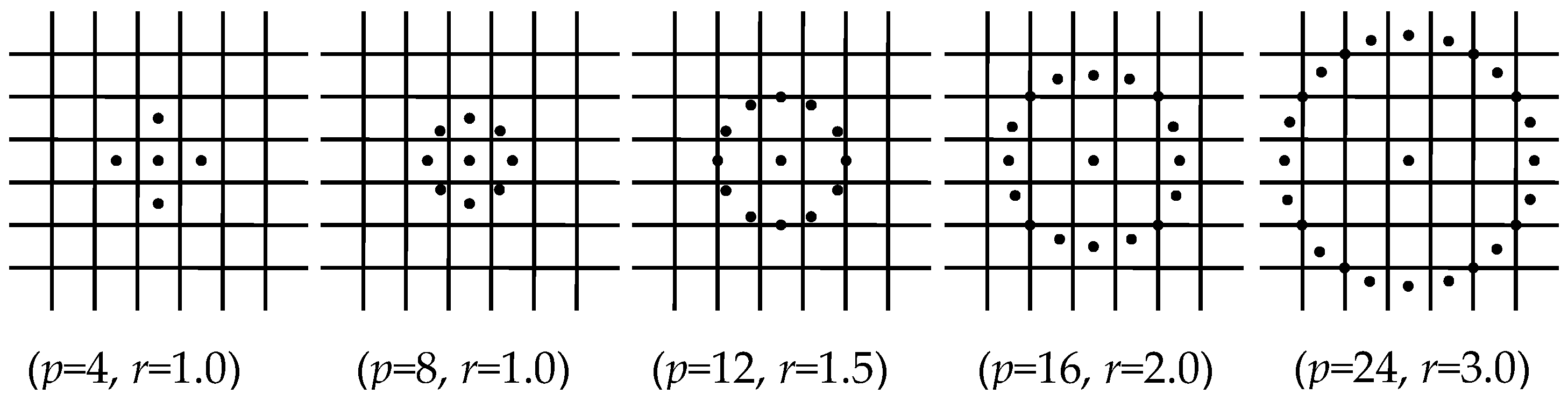
Local Binary Pattern [28] is one of the most common methods in image processing. The LBP operator assigns binary values as a result of comparing them to each other by scrolling floating windows and selecting the center pixel value in the middle of these windows as the threshold level. The generated binary number sequence is called the LBP code, which is used to specify different properties in the image, such as edges, corners, light or dark areas, line regions. The size of the window can be changed according to the problems in order to capture different properties. The length of the LBP code is circularly defined by two parameters, such as the number of sample pixels p and the radius r of the symmetric circular neighborhood as shown in Figure 1. LBPp,r defines the appropriate 2p different output value from the neighboring pixel set.
The histogram of the image is obtained by Equation (1) using LBP. (xc, yc) is the location of the given pixel and ip and ic are the gray level of the center pixel.
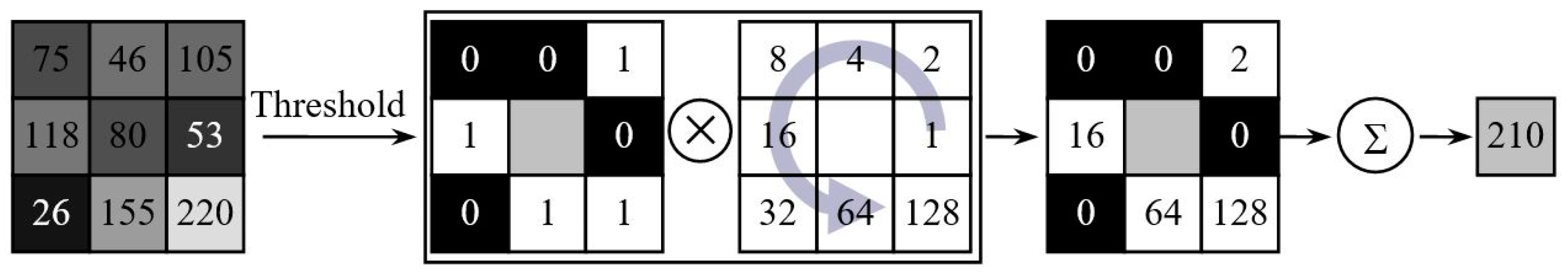
The process of extracting the feature vector (histogram) using the sliding windows of the LBP operator is shown in Figure 2. The center pixel of the window is set as the threshold value using sliding windows. The neighboring pixel values greater than the threshold value assigned to 1 and the small values assigned to 0. The obtained values multiplied by the mask and collected.
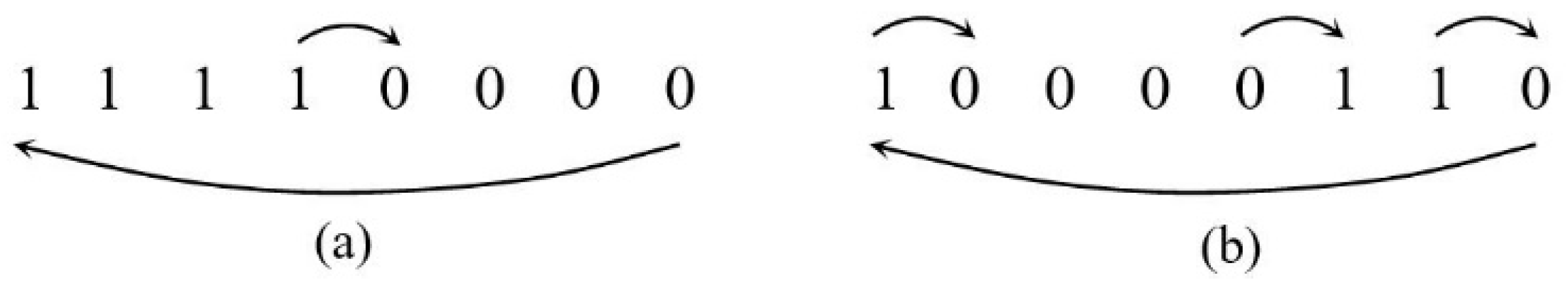
Ojala et al. [22,29] divide LBP codes into two different classes: uniform and non-uniform. A code with a uniform distribution has maximum of 2 times different bits transitions. Examples of uniform and non-uniform LBP code are shown in Figure 3. Figure 3a has 2 transitions; uniform LBP code; Figure 3b is the non-uniform LBP code because it has 4 transitions.
2.2. GP-Descriptor
The GP-descriptor is a GP-based image descriptor, is proposed by Al-Sahaf et al., inspired by the LBP algorithm [30]. The GP-descriptor targets to automatically generate an image descriptor similar to the LBP. As in the standard LBP, the corresponding division of the resulting value in the decimal is increased by 1. The fitness function consists of two components: The classification accuracy and distance. The classification accuracy measures the ability of accurate classification of training instances using the k-NN classifier when evaluating histograms. Distance function calculates distance of between-classes and distance of within classes.
GP-criptor is adopted tree-based GP to represent the solution. GP-criptor is designed to operate directly on image raw pixel values [30]. The criptor uses a sliding window of a predetermined size and the pixel values that fall within the window are used as inputs in the system. Criptor has a special node called code node that represents the root of the program tree. The node uses the input parameters to generate a binary code at each position of the sliding window.
In this paper, ABCP-descriptor was proposed for the first time, inspired by the proposed GP-descriptor in [30], and performance was monitored with two texture datasets.
3. The Proposed Method
This section provides an overview of the overall operation of the ABCP-based image descriptor, the program structure, the terminal and the function set, and the evaluation of the program.
3.1. General Procedure of Algorithm
Each dataset consists of different texture classes, and each texture class consists of multiple instances of small sizes. The data sets are divided into two instances randomly selected as 50% training and 50% test. From the training set, two random instances are selected from each class. The algorithm feeds ABCP using 2 instances from each class in the training phase. By using the fitness function, ABCP solutions are improved and when the stopping criteria is achieved, the ABCP model with the best fitness value is extracted. For each instance in the test set, feature vectors (histograms) are obtained using the best model. Histograms are classified by simple and rapid method 1-Nearest Neighbor (1-NN). The performance of the model is evaluated by the classification success. Details of the steps of the algorithm are presented in the following sections. The steps of the descriptor are given in Figure 4.
3.2. Artificial Bee Colony Programming
ABCP is a high-level automatic programming method based on ABC algorithm [4,31,32]. The steps of the ABCP are similar to the ABC algorithm. The two fundamental differences between these algorithms are the representation of the solution structure and the information sharing mechanism that enables the development of solutions. In ABC, the positions of the food sources, i.e. solutions, are carried out with fixed size arrays and displays the values found by the algorithm for the predetermined variables as in GA. In the ABCP, the positions of food sources are expressed in tree structure that is composed of different combinations of terminals and functions. The smallest unit of trees is called a node. Nodes are selected from the specially defined terminal set (variables such as x, y, variables and constants) and the function set (arithmetic operators, logical functions, mathematical functions). Trees representing the solutions are created with the combination of the nodes. The representation of a solution tree for ABCP is the shown in Figure 5. The mathematical model of the tree in Figure 5 is as in Equation (2) where x and y are defined independent variable and f(x) is dependent variable. The equation of the tree is obtained by combining the terminals and functions in the nodes from the leaves to the root.
The complexity of the solution trees is calculated by Equation (3) in proportion to the number of nodes and the depth of trees.
The flow diagram for the ABCP method is given in Figure 6. As in the GP, solutions at the initial phase in ABCP can be produced with “full”, “grow” and “ramped half and half” methods [3]. The quality of each solution tree is determined by considering the fitness function, which is specifically determined to each problem.
Since solutions are represented by fixed-size arrays in ABC, the candidate solution generation cannot be used directly in ABCP. In order to produce the candidate solution () in the ABCP where solutions are represented tree structures have variable depth and different numbers of nodes, the crossover operator in GP [3] has been adapted to the neighborhood research process on ABC.
In the ABCP algorithm, there three different types of bees: employed bees, onlooker bees and scout bees. Employed bees leave the hives and they have a specific food source in their memory. When they return to the hive, they share information about the food sources with onlooker bees. The onlooker bees decide which source they will go to base on the amount of the nectar of the source shared by the employed bees. During the scout bee phase, it is checked to see whether all food sources are exhausted. If the food source is exhausted, the source is abandoned. The bees formally used with an abandoned source turn into scout bees and search randomly for a new source. Unlike other bees, scout bees find new food sources without sharing information. The exhausted of food resources controls a parameter called “limit”. For each source, the number of improving trials is kept, and in each cycle, it is checked to see whether the number of trials exceeds the “limit” parameter.
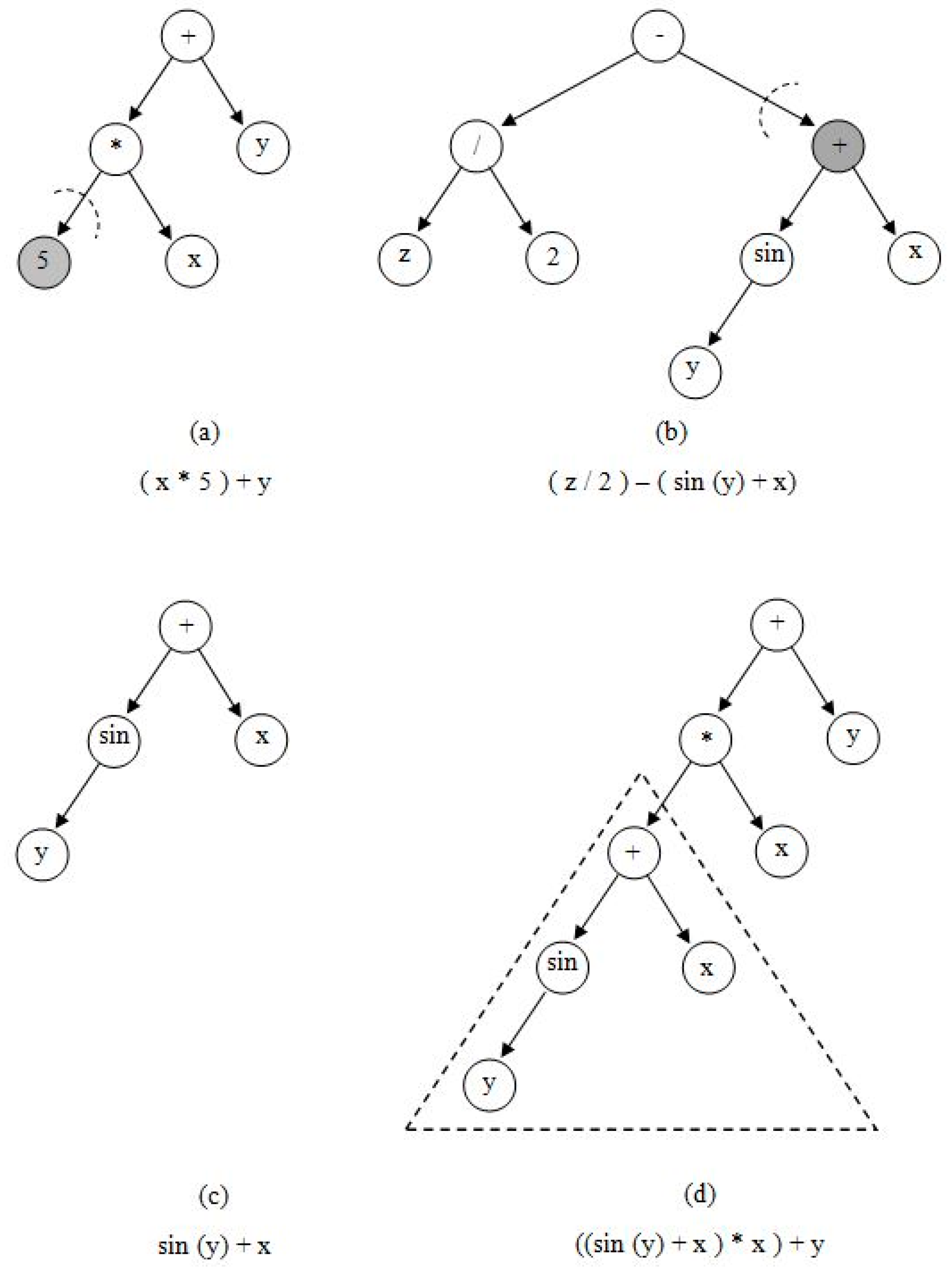
When generating the candidate solution , the neighbor node solution (), taken from a different solution in the population is randomly selected as a mechanism considering the probability of . The node is randomly selected from the neighbor solution and determines what information to share in the current solution. Similarly, a function node is selected in the probability of (set to 0.9) and a terminal in the probability of (1−) is selected from the current solution . The candidate solution is generated by replacing the nodes of the current solution node and the neighbor solution node . This sharing mechanism is shown in Figure 7. Figure 7a,b are node representing the current solution and a neighbor node taken from the tree respectively, Figure 7c shows neighboring information and the generated candidate solution is given in Figure 7d. After the candidate solution is generated, a greedy selection process is applied between the node expressing the current solution and the candidate solution . The candidate solution is evaluated, and greedy selection is used for each employed bee.
3.3. ABCP-Descriptor Program Representation
ABCP-descriptor is an ABCP-based image descriptor that generates models using raw pixel values. The descriptor presents the pixel values in a certain size of sliding windows. The pixel values are used inputs of a feature vector. Figure 8 shows representation of the feature vector. In the example in Figure 8, window size 5 × 5 is selected. The window has a value of 5 × 5 = 25 pixels. The first pixel is labelled with P0 and is labeled up to P24 in total. Pixels are sequenced from left to right and feature vector is generated. Therefore, the inputs of the ABCP are (P0, P1, …, P24) in feature vector.
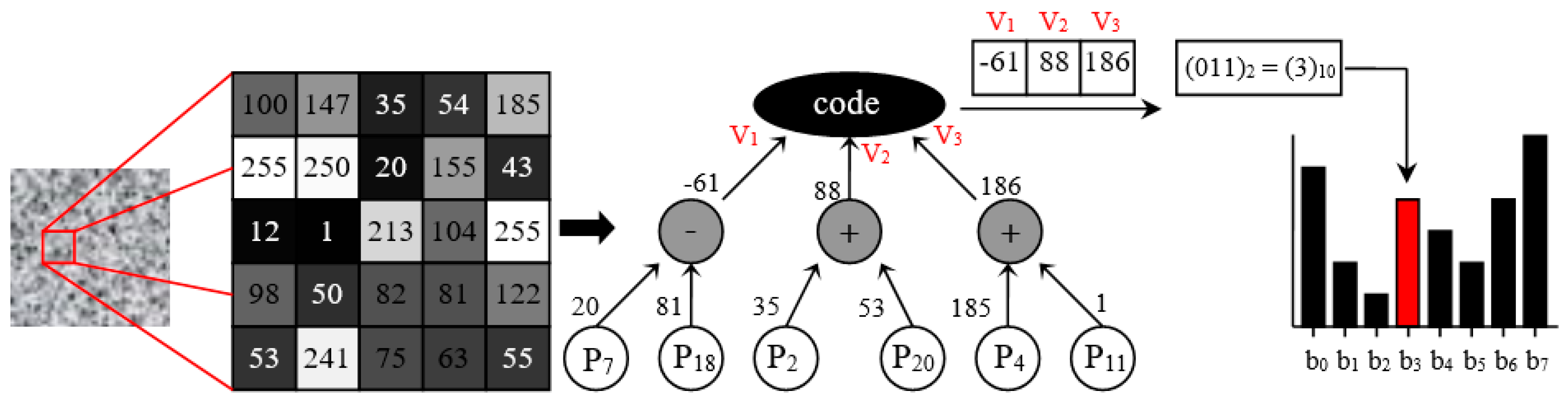
The ABCP function set consists of simple arithmetic operators {+, -, *, /} and the code root node. The divide (/) function in the function set is a protected version where the divisor value is equal to 0, it is later revised to 1, otherwise, normal division is performed. The code node creates binary code using the inputs in row vectors. The number of children of the code node determines the length and range of the generated code. For example, if the number of children is 5, the length of the binary code is 5 bits and the program can produce different values up to 25 = 32 (0.1, …, 31). The representation of the ABCP-descriptor is given in Figure 9.
As shown in Figure 9, the sliding window is selected as 5 * 5 and has 25 inputs. Since the code node has 3 children, the resulting feature vector can produce 23=8 different values. If the values obtained from the branches of the code node are greater than 0, the binary code is converted into 1 and if it is less than 0 the binary code is converted into 0. In the program representation, the binary code is obtained as (011)2. The code is converted to decimal and the value of the partition in the feature vector (histogram) is increased by 1. For example, a histogram of the model is obtained by moving the sliding window over the instance. In the process of ABCP-descriptor, 2 instances are selected for each class, c is defined class number and 2 *c histogram is obtained. The test instances are classified by taking into account the distances between the histograms obtained in the training instances and the histograms of the test instances generated with the best model.
3.4. Fitness Function
In this paper, only a few random instances are selected from the training set and the classification success is evaluated only after the training of the instances. Therefore, it is aimed to obtain more information from the instances. The classification accuracy is not used as a fitness function alone in order to avoid models over-fitting training instances. Instead, the fitness function that evaluates the distance along with the classification accuracy. To make a reliable and fair comparison, same parameter values are chosen as in [29] and the fitness function (objective function) is adapted as defined in Equation (4).
The classification accuracy is obtained by the ratio of the number of correctly classified instances to the total number of instances. Accuracy is defined Equation (5).
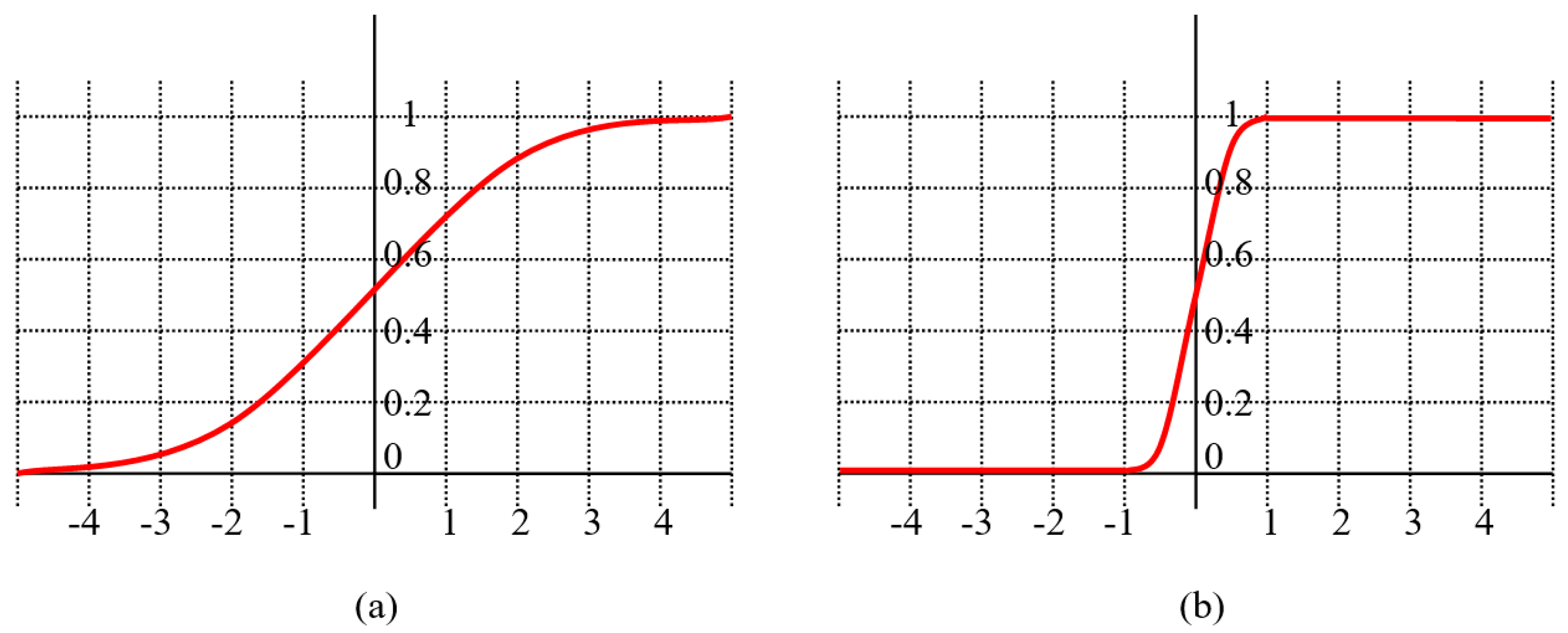
Ncorrect is the number of correctly classified instances and Ntotal is the total number of instances. Distance is the function that calculates the distance between classes and the distance within classes. Since the logical function range is in the range [–5, 5], the range of [–1, 1] has been adjusted by adapting the function. The representation of the logical function is given in Figure 10.
The logical function shown in Figure 10a is defined Equation (6); Figure 10b is defined Equation (7).
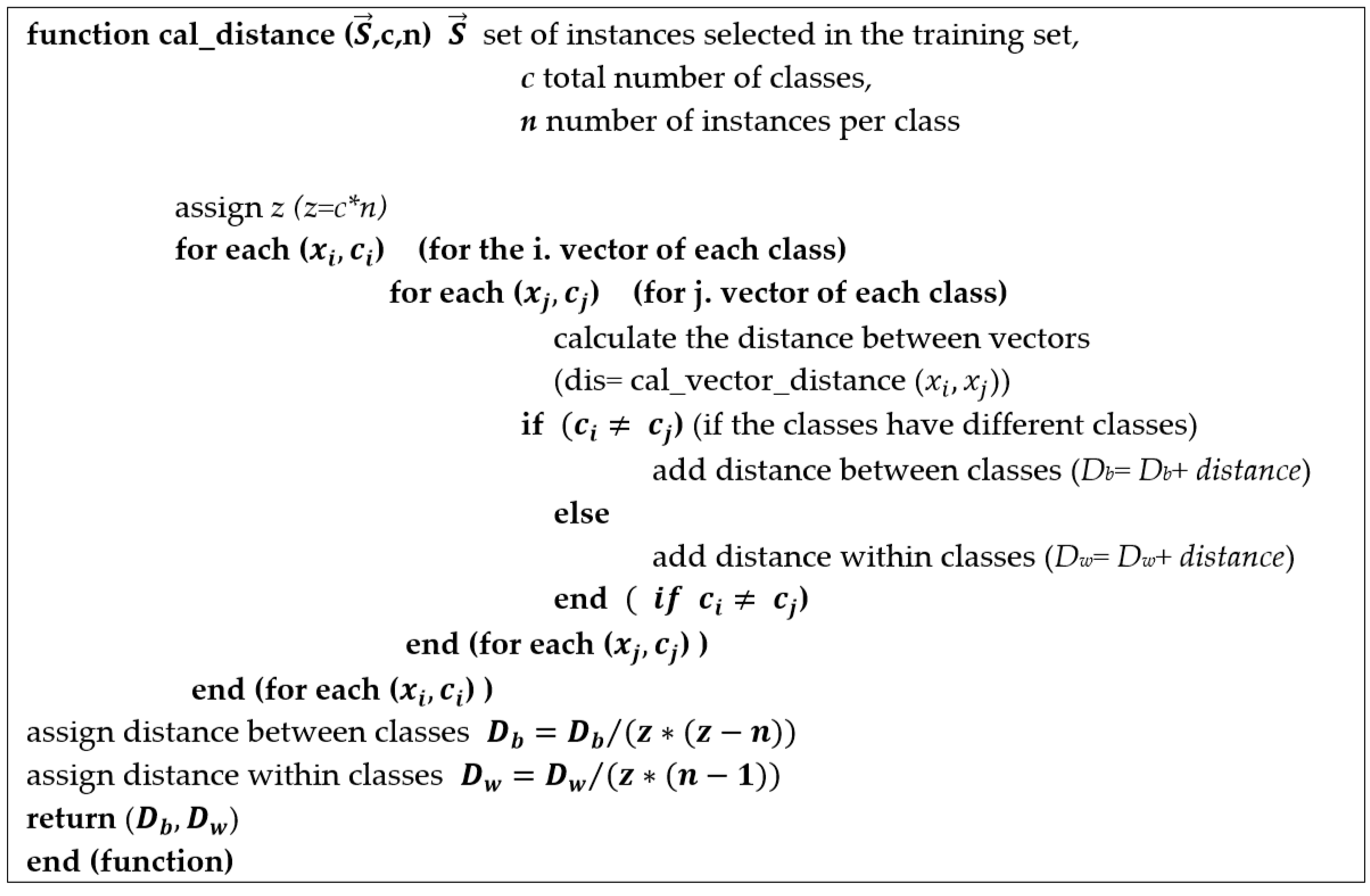
Adapted version of the distance function according to the logical function (Equation (7)) is shown in Equation (8). Db (between distances) calculates the average distance between classes, and Dw (within Distances) calculates the average distance within classes. Db and Dw, respectively are defined in Equations (9) and (10).
where the set of instances is selected in the training set, is the feature vector of each instance, and is the class label. ; c and n respectively define the total number of classes and the number of instances per class. The total number of instances in the training set is z (c*n); xα is all instances of the class in Str. The distance between vectors with two normalized equal number of elements is shown in Equation (11).
where ui and vi, respectively are defined i. element is u and v vectors. If the divisor of Equation (11) is 0, the protected function returns 0 as a result. The classification accuracy (Equation (5)) and the distance (Equation (8)) take the value 1 in the best case and 0 in the worst case. Therefore, the fitness function (Equation (4)) for the automatic programming method can be defined as a minimization problem.
In summary, the following steps are followed to extract the feature vector from the image descriptor.
- Step 1. Instances are converted to feature vectors of the previously defined window size (for example 5*5). (Figure 8)
- Step 2. Leaf nodes are fed the root code node and the binary status of the branches is checked by checking the negativity of the branches.
- Step 3. By converting the binary code to the decimal, the corresponding value of the number is increased by 1 in the histogram.
- Step 4. Using histograms of instances.
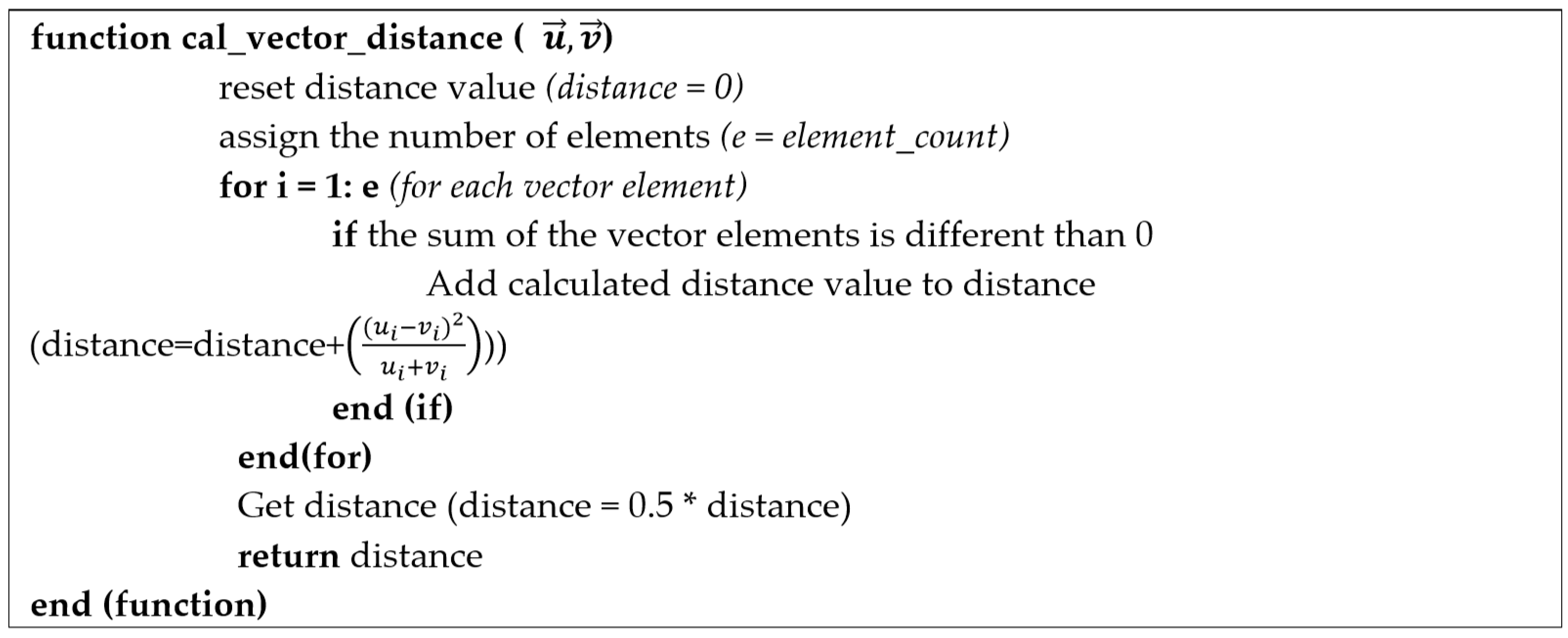
Calculation of distance between vectors (Figure 11)
The fitness values of the trees (individuals) are calculated.
- Step 5. The ABCP algorithm (Figure (6)) is operated according to the fitness values.
Pseudo-Code 1 calculates the distance between vectors (Equation (11)), shown in Figure 11.
ABCP-descriptor is expected to improve the trees according to their fitness values. When stopping criteria are provided, the best individual is classified in test data.
4. Experimental Design
For the performance analysis of the proposed method, experiments were conducted using two different datasets and the results were evaluated. This section provides detailed information about the parameters used in datasets and automatic programming methods.
4.1. Datasets
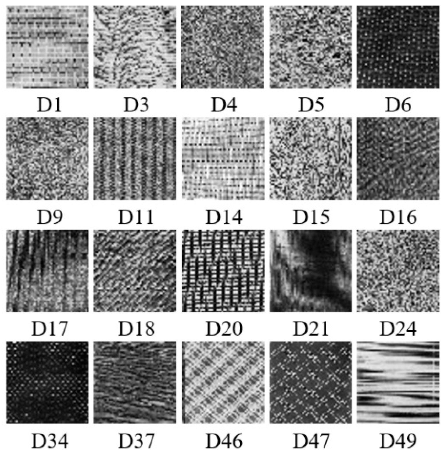
The methods were tested on two different texture datasets DS-Broadtz (Dover Publications, New York, NY, USA) and DS-Kylberg (Swedish University of Agricultural Sciences, Uppsala, Sweden) which are commonly used in image processing. To compare with [29], we selected the same classes in both texture datasets in [30]. The first dataset DS-Broadtz was obtained from the Broadtz texture set [33]. The original set consists of 112 classes, each 640*640 pixels. In this paper, 20 classes of 112 class are compared. Texture instances of the selected classes are shown in Figure 13. Texture instances of each class are divided into 64*64 pixel samples and 100 instances are obtained.
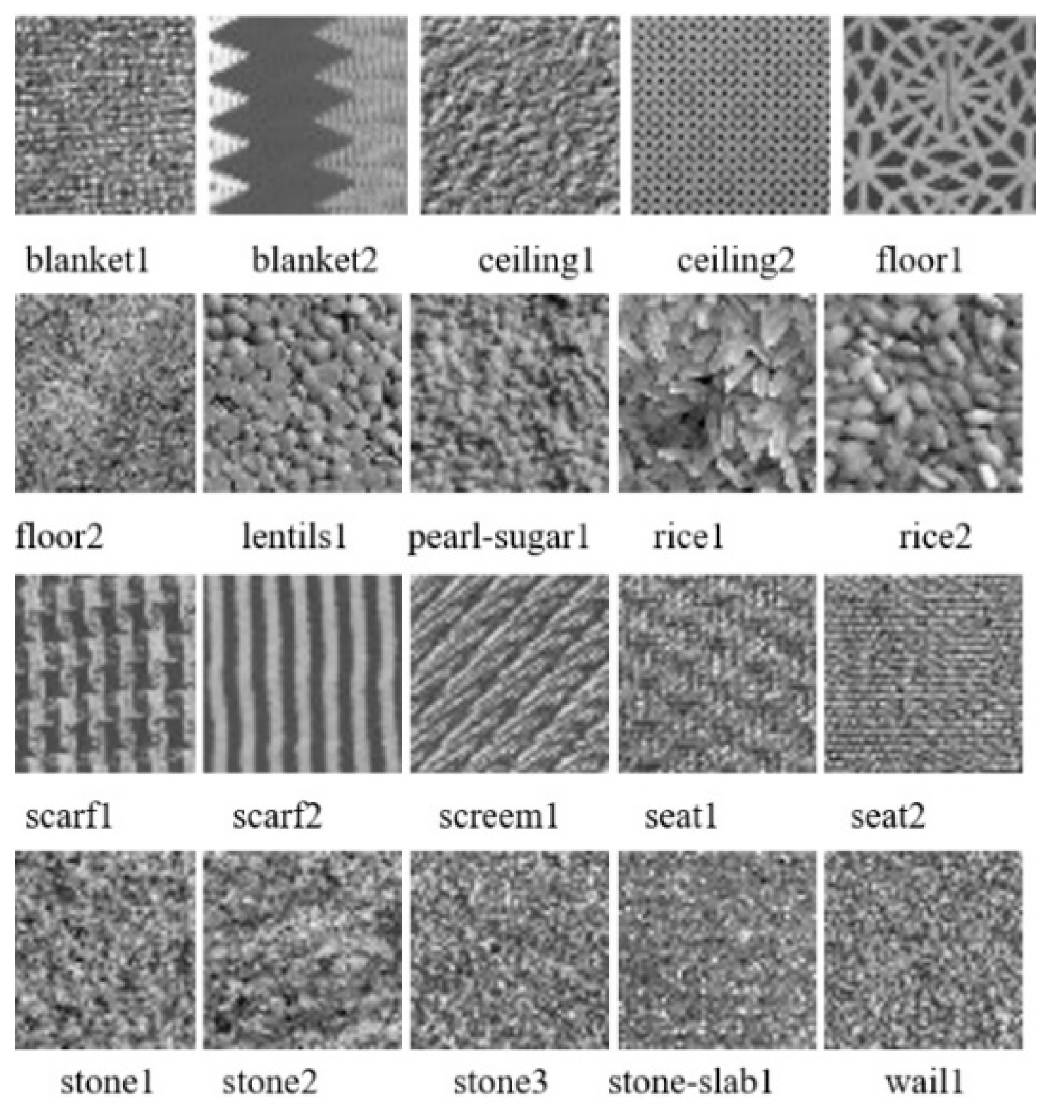
The second dataset DS-Kylberg was obtained from the Kylberg dataset [34]. The Kylberg dataset is divided into two parts, originally rotated and non-rotated. As in the Broadtz dataset from the non-rotated Kylberg data set, 20 selected classes were used. Each class contains 160 instances with 576* 576 pixels. In this paper, each instance was reduced to 115 *115 pixels in order to reduce the cost of calculation. Texture instance samples of the selected Kylberg dataset are shown in Figure 14.
Table 1 shows the total number of selected classes (Nclasses) from the Broadtz and Kylberg datasets, the number of instances contained in each class (Ninstances), the number of instances used in the training and test (Ntrain_in , Ntest_in) and the instance dimensions (width* height).
As shown in Table 1, DS-Broadtz has 1000 instances (20 classes*50 instances); DS-Kylberg used 1600 instances (20 classes*50 instances) in total for training and testing.
4.2. Parameters
The parameter values of the ABCP-descriptor are shown in Table 2. In all methods, the initial solutions are produced with Ramped Half and Half method. In order to increase the quality of sources in the descriptor, Information Sharing Mechanism was used in all solutions. The number of sub-trees / branches connected to the code node has a fixed number of 7. Thus, the histogram can have 27 = 128 different values (0, 1, …, 127). The division (/) function in the function set is the protected version. In this function, if the divisor value is equal to 0, then 1 is returned, in other cases normal division is performed. p and r are assigned respectively 8 and 1 for the LBPp,r operator. In this paper, the limit parameter was set to half of the colony size in ABCP-criptor. When the limit is exceeded, the abandoned food source is randomly changed with a new food source. The identifier does not use weight for subtrees. The maximum depth of the subtrees is set to 6.
5. Performance Analysis
The experimental results of the methods are given and discussed in this section. ABCP-descriptor and LBP8,1 were run 10 times independently. In each run, the methods analyzed randomly selected instances from datasets and tried to assign test instances to the correct texture class. We evaluated the ability to learn the descriptors in the training set.
5.1. Overall Results
The simulation results for ABCP-descriptor, LBP8,1 and GP-descriptor [30] are presented in Table 3. In [30] is tested the performance of GP-criptor against nine of the widely used classical methods in machine learning. The performances of the methods are significantly low compared to that of GP-criptor. For this reason, we compared the results with the GP-criptor [30] by proposing the ABCP-criptor, which is a new method that can rival the GP-criptor, which has a higher result than the classical methods.
When the results were evaluated, successful results were obtained with ABCP-descriptor and LBP. The average test success of the methods in the DS-Broadtz is higher than the DS-Kylberg. The highest test accuracy was found in the ABCP-descriptor as 97.3% for the DS-Broadtz and 95.188 for the DS-Kylberg. The highest standard deviation has the ABCP-descriptor in the DS-Kylberg data set with 6.38. The higher the deviation, the greater the difference between the maximum and the minimum test accuracy compared to LBP. The GP-descriptor [30] has the highest mean as 93.21% in DS-Kylberg. The ABCP-descriptor is considered to be comparable to the GP-descriptor because its classification success is high.
5.2. Model Analysis Results
In this section, the best models of test accuracy with ABCP-descriptor for each dataset will be analyzed.
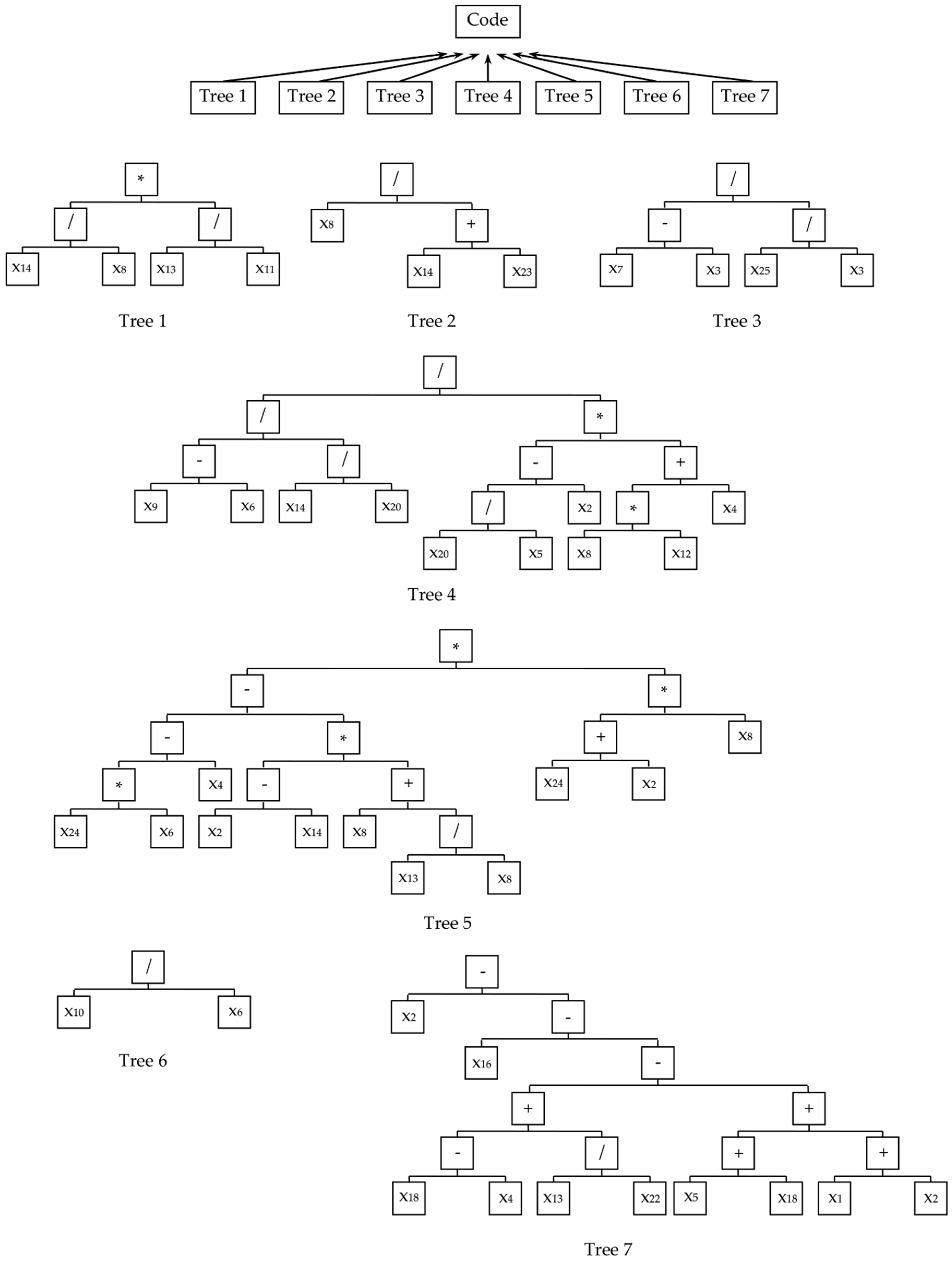
Table 4 shows the general information about the parse trees of the best model with has highest test classification with 97.3% in DS_Broadtz. The complexity in Table 4 was calculated according to Equation (3). As shown in the table, the sub-trees connected to the code node depend on different depth and number of nodes. A tree representation of the model test success for the DS-Broadtz dataset is shown in Table 5. The equations of the sub-trees of the best model in Figure 15 is shown in Table 6.
A tree representation of the model test success for the DS-Kylberg dataset is shown in Figure 16. The equations of the sub-trees of the best model in Figure 16 are shown in Table 7. When the tables of the highest classification test accuracy for the DS-Kylberg dataset (Table 6, Table 7) are evaluated, it can be seen that the sub-trees of the model are more complex than the best model sub-trees of DS-Broadtz. Many inputs in the lower trees (such as x14, x15, x20) are common in the model. The code node of the best models for both datasets have 7 subtrees and the trees have depth of 2-6. As the number of nodes and depth of the tree increase, the tree complexity increases.
6. Conclusions
In this paper, ABCP-descriptor is proposed to identify texture by selecting only two instances randomly in the training set for each texture. In the proposed method, the instances were transformed into feature vectors using a window of 5*5 dimensions. Feature vectors were used as inputs for models in the ABCP-descriptor. Similar to LBP algorithm, the binary codes obtained by the models are converted to decimal and the corresponding value is increased by 1 in the histogram. The fitness function in the descriptor is composed of two components: classification accuracy and distance. The classification accuracy measures the ability to accurately classify training instances using the 1-NN classifier when evaluating histograms. The distance function calculates the distance between classes and within classes in the training set. ABCP-descriptor is evaluated performance to standard LBP and GP-descriptor. The comparative results show that ABCP-descriptor is a new method that can be used in this field. In the future, we aim to test the success of classification of models using different tree sizes and different arithmetic functions (such as sin, cos etc.). In addition, attempts will be made to extract new models will by changing the parameters, rotated textures.
Author Contributions
All sections are implemented and written S.A. and C.O.
Funding
This research received no external funding.
Conflicts of Interest
The authors declare no conflict of interest.
References
- Liu, L.; Zhao, L.; Long, Y.; Kuang, G.; Fieguth, P. Extended Local Binary Patterns for Texture Classification. Image Vis. Comput. 2012, 30, 86–99. [Google Scholar] [CrossRef]
- Biermann, A.W. Automatic Programming: A Tutorial on Formal Methodologies. J. Symb. Comput. 1985, 1, 119–142. [Google Scholar] [CrossRef]
- Koza, J.R. Genetic Programming: On the Programming of Computers by Means of Natural Selection; MIT Press: Cambridge, MA, USA, 1992; Volume 4, pp. 87–112. [Google Scholar]
- Karaboga, D.; Ozturk, C.; Karaboga, N.; Gorkemli, B. Artificial Bee Colony Programming for Symbolic Regression. Inf. Sci. 2012, 209, 1–15. [Google Scholar] [CrossRef]
- Tackett, W.A. Genetic Programming for Feature Discovery and Image Discrimination. In Proceedings of the 5th International Conference on Genetic Algorithms, Urbana, IL, USA, 17–21 July 1993; pp. 303–311. [Google Scholar]
- Shao, L.; Liu, L.; Li, X. Feature Learning for Image Classification via Multiobjective Genetic Programming. IEEE Trans. Neural Netw. Learn. Syst. 2014, 25, 1359–1371. [Google Scholar] [CrossRef]
- Lensen, A.; Sahaf, H.A.; Zhang, M.; Xue, B. A Hybrid Genetic Programming Approach to Feature Detection and Image Classification. In Proceedings of the International Conference on Image and Vision Computing, New Zealand (IVCNZ), Auckland, New Zealand, 23–24 November 2015. [Google Scholar]
- Iqbal, M.; Xue, B.; Al-Sahaf, H.; Zhang, M. Cross-Domain Reuse of Extracted Knowledge in Genetic Programming for Image Classification. IEEE Trans. Evol. Comput. 2017, 21. [Google Scholar] [CrossRef]
- Lensen, A.; Al-Sahaf, H.; Zhang, M.; Xue, B. Genetic Programming for Region Detection, Feature Extraction, Feature Construction and Classification in Image Data. In Proceedings of the European Conference on Genetic Programming EuroGP Genetic Programming, Porto, Portugal, 30 March–1 April 2016; pp. 51–67. [Google Scholar]
- Al-Sahaf, H.; Song, A.; Neshatian, K.; Zhang, M. Two-Tier Genetic Programming: Towards Raw Pixel-Based Image Classification. Expert Syst. Appl. 2012, 39, 12291–12301. [Google Scholar] [CrossRef]
- Karaboga, D.; Basturk, B. On the Performance of Artificial Bee Colony (ABC) Algorithm. Appl. Soft Comput. 2008, 8, 687–697. [Google Scholar] [CrossRef]
- Hancer, E.; Ozturk, C.; Karaboga, D. Artificial Bee Colony Based Image Clustering Method. In Proceedings of the WCCI IEEE World Congress on Computational İntelligence, Brisbane, Australia, 10–15 June 2012; pp. 10–15. [Google Scholar]
- Wang, S. Artificial Bee Colony used for Rigid Image Registration. Int. J. Res. Rev. Soft Intell. Comput. (Ijrrsic) 2011, 1, 1936–1953. [Google Scholar]
- Karaboga, D.; Ozturk, C. Neural Networks Training by Artificial Bee Colony Algorithm on Pattern Classification. Neural Netw. World 2009, 19, 279–292. [Google Scholar]
- Maa, M.; Lianga, J.; Guoa, M.; Fana, Y.; Yinb, Y. SAR Image Segmentation Based on Artificial Bee Colony Algorithm. Appl. Soft Comput. 2011, 11, 5205–5214. [Google Scholar] [CrossRef]
- Hu, Z.; Yu, W.; Lv, S.; Feng, J. Multi-level threshold Image Segmentation Using Artificial Bee Colony Algorithm. In Proceedings of the Fifth Conference on Measuring Technology and Mechatronics Automation, Hong Kong, China, 16–17 January 2013. [Google Scholar]
- Dakshitha, B.A.; Deekshitha, V.; Manikantan, K. A Novel Bi-Level Artificial Bee Colony Algorithm and Its Application to Image Segmentation. In Proceedings of the IEEE International Conference on Computational Intelligence and Computing Research (ICCIC), Madurai, India, 10–12 December 2015. [Google Scholar]
- Sag, T.; Cunkas, M. Color Image Segmentation Based on Multiobjective Artificial Bee Colony Optimization. Appl. Soft Comput. 2015, 34, 389–401. [Google Scholar] [CrossRef]
- Hancer, E.; Ozturk, C.; Karaboga, D. Extraction of Brain Tumors from MRI Images with Artificial Bee Colony Based Segmentation Methodology. In Proceedings of the 8th International Conference on Electrical and Electronics Engineering (ELECO), Bursa, Turkey, 28–30 November 2013. [Google Scholar]
- Agrawal, V.; Chandra, S. Feature Selection Using Artificial Bee Colony Algorithm for Medical Image Classification. In Proceedings of the Eighth International Conference on Contemporary Computing (IC3), Noida, India, 20–22 August 2015. [Google Scholar]
- Al-Sahaf, H.; Zhang, M.; Johnston, M. Binary Image Classification Using Genetic Programming Based on Local Binary Patterns. In Proceedings of the 28th International Conference on Image and Vision Computing, Wellington, New Zealand, 27–29 November 2013. [Google Scholar]
- Ojala, T.; Pietikaè, M.; Maèenpaè, T. Multiresolution Gray-Scale and Rotation Invariant Texture Classification with Local Binary Patterns. IEEE Trans. Pattern Anal. Mach. Intell. 2002, 24, 971–981. [Google Scholar] [CrossRef]
- Sinha, A.; Banerji, S.; Liu, C. Scene Image Classification Using a Wigner-Based Local Binary Patterns Descriptor. In Proceedings of the 2014 International Joint Conference on Neural Networks (IJCNN), Beijing, China, 6–11 July 2014. [Google Scholar]
- Pan, Z.; Li, Z.; Fan, H.; Wu, X. Feature Based Local Binary Pattern for Rotation Invariant Texture Classification. Expert Syst. Appl. 2017, 88, 238–248. [Google Scholar] [CrossRef]
- Bunna, N. Multi-Class Object Classification and Detection Using Neural Networks. BSc Honours Research, Project/Thesis, School of Mathematical and Computing Sciences, Victoria University of Wellington, Wellington, New Zealand, October 2003. [Google Scholar]
- Zhang, M.; Ciesielski, V. Using back propagation algorithm and genetic algorithm to train and refine neural networks for object detection. In Lecture Notes in Computer Science, Proceedings of the 10th International Conference on Database and Expert Systems Applications (DEXA’99), Florence, Italy, 30 August–3 September 1999; Bench-Capon, T., Soda, G., Tjoa, A.M., Eds.; Springer: Berlin, Germany, 1999; LNCS Volume 1677, pp. 626–635. [Google Scholar]
- Zhang, M.; Bhowan, U.; Ny, B. Genetic programming for object detection: A two-phase approach with an improved fitness function. Electron. Lett. Comput. Vis. Image Anal. 2007, 6, 27–43. [Google Scholar] [CrossRef]
- Ojala, T.; Pietikäinen, M.; Harwood, D. Performance Evaluation of Texture Measures with Classification Based on Kullback Discrimination of Distributions. In Proceedings of the 12th International Conference on Pattern Recognition, Jerusalem, Israel, 9–13 October 1994; Volume 1, pp. 582–585. [Google Scholar]
- Ojala, T.; Pietikäinen, M.; Mäenpää, T. Gray Scale and Rotation Invariant Texture Classification with Local Binary Patterns. In Proceedings of the European Conference on Computer Vision, Dublin, Ireland, 26 June–1 July 2000; pp. 404–420. [Google Scholar]
- Al-Sahaf, H.; Zhang, M.; Johnston, M.; Verma, B. Image Descriptor: A Genetic Programming Approach to Multiclass Texture Classification. In Proceedings of the 2015 IEEE Congress on Evolutionary Computation (CEC), Sendai, Japan, 25–28 May 2015; pp. 2460–2467. [Google Scholar]
- Gorkemli, B.; Ozturk, C.; Karaboga, D. Yapay Arı Kolonisi Programlama ile Sistem Modelleme. In Proceedings of the Otomatik Kontrol Türk Milli Komitesi 2012 Ulusal Toplantısı (TOK), Niğde, Turkey, 11–13 October 2012; pp. 857–860. [Google Scholar]
- Arslan, S.; Ozturk, C. Multi Hive Artificial Bee Colony Programming for high dimensional symbolic regression with feature selection. Appl. Soft Comput. J. 2019, 78, 515–527. [Google Scholar] [CrossRef]
- Brodatz, P. Textures: A Photographic Album for Artists and Designers; Dover: New York, NY, USA, 1999. [Google Scholar]
- Kylberg, G. The Kylberg Texture Dataset V. 1.0; Technical Report 35; Centre Image Anal., Swedish University of Agricultural Sciences: Uppsala, Sweden, 2011. [Google Scholar]
Figure 1.
LBP parameter samples.

Figure 2.
Example of converting LBP code to decimal.

Figure 3.
Uniform and non-uniform LBP code examples; (a) uniform LBP; (b): non-uniform LBP

Figure 4.
General mechanism of descriptor.

Figure 5.
Representation of solutions in ABCP by tree structure.

Figure 6.
Flowchart ABCP algorithm.

Figure 7.
Information sharing mechanism of ABCP algorithm. (a): ; (b): (c): neighbor information (d): generated candidate solution
Figure 7.
Information sharing mechanism of ABCP algorithm. (a): ; (b): (c): neighbor information (d): generated candidate solution

Figure 8.
Row feature vector representation.

Figure 9.
ABCP program representation.

Figure 10.
Logical Functions; (a): logical function range is in the range [–5, 5], (b): logical function range is in the range [–1, 1].
Figure 10.
Logical Functions; (a): logical function range is in the range [–5, 5], (b): logical function range is in the range [–1, 1].

Figure 11.
Calculation of the distance between two vectors is the pseudo code.

Figure 12.
Calculation of between classes and within classes distance pseudo code.

Figure 13.
Instances samples of DS-Broadtz dataset.

Figure 14.
Instances samples of DS-Kylberg dataset.

Figure 15.
Best Model of ABCP-Descriptor for DS-Broadtz.

Figure 16.
Best Model of ABCP-Descriptor for DS-Kylberg.


Table 1.
Datasets.
| Dataset | Nclasses | Ninstances | Ntrain_in | Ntest_in | Instance Dimensions |
|---|---|---|---|---|---|
| Broadtz | 20 | 100 | 50 | 50 | 64*64 |
| Kylberg | 20 | 160 | 80 | 80 | 115*115 |
Table 2.
Parameters.
| Parameters | Artificial Bee Colony Programming-Descriptor (ABCP-Descriptor) |
|---|---|
| Colony Size | 100 |
| Iteration Number | 30 |
| Maximum Tree Depth | 6 |
| Number of Branches in the Code node | 7 |
| Initial Method | Ramped Half and Half |
| Functions | + (plus), −(minus), ∗ (times), / (rdivide) |
| Limit | 50 |
Table 3.
Simulation results of descriptor.
| Descriptor | Dataset | Criteria | Best Test Fitness | Test Classification Success (%) |
|---|---|---|---|---|
| ABCP-descriptor | Broadtz | Mean | 0.03 | 94.55 |
| Maximum | 0.03 | 97.3 | ||
| Minimum | 0.01 | 93.3 | ||
| Standard deviation | 0.01 | 1.17 | ||
| Kylberg | Mean | 0.05 | 89.71 | |
| Maximum | 0.14 | 95.19 | ||
| Minimum | 0.02 | 71.63 | ||
| Standard deviation | 0.03 | 6.38 | ||
| LBP8.1 | Broadtz | Mean | 90.63 | |
| Maximum | 93.8 | |||
| Minimum | 87.3 | |||
| Standard deviation | 1.92 | |||
| Kylberg | Mean | 90 | ||
| Maximum | 93.13 | |||
| Minimum | 87.13 | |||
| Standard deviation | 1.9 | |||
| GP-descriptor [30] | Broadtz | Mean | 94.40 | |
| Standard deviation | 0.81 | |||
| Kylberg | Mean | 93.21 | ||
| Standard deviation | 1.14 | |||
Table 4.
Information about Subtrees of Best Model of ABCP-Descriptor for DS-Broadtz.
| Node | Depth | Complexity | |
|---|---|---|---|
| Tree 1 | 7 | 3 | 17 |
| Tree 2 | 5 | 3 | 11 |
| Tree 3 | 7 | 3 | 17 |
| Tree 4 | 19 | 5 | 69 |
| Tree 5 | 21 | 6 | 83 |
| Tree 6 | 3 | 2 | 5 |
| Tree 7 | 19 | 6 | 87 |
Table 5.
Equations of Subtrees of Best Model of ABCP-Descriptor for DS-Broadtz.
| Equation | |
|---|---|
| Tree 1 | |
| Tree 2 | |
| Tree 3 | |
| Tree 4 | |
| Tree 5 | |
| Tree 6 | |
| Tree 7 |
Table 6.
Information about Subtrees of Best Model of ABCP-Descriptor for DS-Kylberg.
| Node | Depth | Complexity | |
|---|---|---|---|
| Tree 1 | 5 | 3 | 11 |
| Tree 2 | 7 | 3 | 17 |
| Tree 3 | 3 | 2 | 5 |
| Tree 4 | 13 | 6 | 51 |
| Tree 5 | 9 | 4 | 27 |
| Tree 6 | 33 | 6 | 145 |
| Tree 7 | 11 | 4 | 33 |
Table 7.
Equations of Subtrees of Best Model of ABCP-Descriptor for DS-Kylberg.
| Equation | |
|---|---|
| Tree 1 | |
| Tree 2 | |
| Tree 3 | |
| Tree 4 | |
| Tree 5 | |
| Tree 6 | |
| Tree 7 |
© 2019 by the authors. Licensee MDPI, Basel, Switzerland. This article is an open access article distributed under the terms and conditions of the Creative Commons Attribution (CC BY) license (http://creativecommons.org/licenses/by/4.0/).
Share and Cite
MDPI and ACS Style
Arslan, S.; Ozturk, C. Artificial Bee Colony Programming Descriptor for Multi-Class Texture Classification. Appl. Sci. 2019, 9, 1930. https://doi.org/10.3390/app9091930
AMA Style
Arslan S, Ozturk C. Artificial Bee Colony Programming Descriptor for Multi-Class Texture Classification. Applied Sciences. 2019; 9(9):1930. https://doi.org/10.3390/app9091930
Chicago/Turabian StyleArslan, Sibel, and Celal Ozturk. 2019. "Artificial Bee Colony Programming Descriptor for Multi-Class Texture Classification" Applied Sciences 9, no. 9: 1930. https://doi.org/10.3390/app9091930
Note that from the first issue of 2016, this journal uses article numbers instead of page numbers. See further details here.