
Assessing Multi-Temporal Global Urban Land-Cover Products Using Spatio-Temporal Stratified Sampling

1
College of Surveying and Geo-Informatics, Tongji University, Shanghai 200092, China
2
Shanghai Key Laboratory of Space Mapping and Remote Sensing for Planetary Exploration, Tongji University, Shanghai 200092, China
3
Shanghai Institute of Intelligent Science and Technology, Tongji University, Shanghai 200092, China
*
Author to whom correspondence should be addressed.
ISPRS Int. J. Geo-Inf. 2022, 11(8), 451; https://doi.org/10.3390/ijgi11080451
Submission received: 9 June 2022
/
Revised: 26 July 2022
/
Accepted: 13 August 2022
/
Published: 19 August 2022
Abstract
:In recent years, the availability of multi-temporal global land-cover datasets has meant that they have become a key data source for evaluating land cover in many applications. Due to the high data volume of the multi-temporal land-cover datasets, probability sampling is an efficient method for validating multi-temporal global urban land-cover maps. However, the current accuracy assessment methods often work for a single-epoch dataset, and they are not suitable for multi-temporal data products. Limitations such as repeated sampling and inappropriate sample allocation can lead to inaccurate evaluation results. In this study, we propose the use of spatio-temporal stratified sampling to assess thematic mappings with respect to the temporal changes and spatial clustering. The total number of samples in the two stages, i.e., map and pixel, was obtained by using a probability sampling model. Since the proportion of the area labeled as no change is large while that of the area labeled as change is small, an optimization algorithm for determining the sample sizes of the different strata is proposed by minimizing the sum of variance of the user’s accuracy, producer’s accuracy, and proportion of area for all strata. The experimental results show that the allocation of sample size by the proposed method results in the smallest bias in the estimated accuracy, compared with the conventional sample allocation, i.e., equal allocation and proportional allocation. The proposed method was applied to multi-temporal global urban land-cover maps from 2000 to 2010, with a time interval of 5 years. Due to the spatial aggregation characteristics, the local pivotal method (LPM) is adopted to realize spatially balanced sampling, leading to more representative samples for each stratum in the spatial domain. The main contribution of our research is the proposed spatio-temporal sampling approach and the accuracy assessment conducted for the multi-temporal global urban land-cover product.
1. Introduction
With the rapid development of remote sensing technology and free data access, more and more land-cover maps have been produced via image classification analysis in recent decades [1]. Such products are important for environmental monitoring applications, such as studies of water-related ecosystems, urban land expansion, the loss of cultivated land, and deforestation [2]. However, different types of errors and uncertainties are encountered during the process of generating land-cover data; in the acquisition, processing, classification, and analysis of the data [3,4,5]; and the impact of these errors directly affects the quality of the final product. Thus, an unbiased estimation of the accuracy of the land-cover products is necessary.
In previous research studies, accuracy assessment has been used to validate land-cover products and provide the user with a better understanding of the product quality [6]. The result of the accuracy assessment can also help producers in improving the classifier, seek optimized classification features, or combine external data to improve the classification’s accuracy [7]. The main process of accuracy assessment is quantifying the spatial and attribute consistency between the classification product and the reference data [6]. According to the principles of statistics, several representative sample points can be chosen in geographic space, and corresponding reference data that can reflect the ground truth are selected [8]. The reference labels can then be visually interpreted from very high-resolution data, such as aerial photographs or field measurement data [9]. The implementation of statistically rigorous accuracy assessment can, thus, be achieved based on good practices [10] and sampling-based estimation, reflecting the consistency of the map classification and reference data [11]. An error matrix is a cross-tabulation of map classification labels against reference data labels. Its rows represent the map classification labels and the columns represent reference data labels. Then, the corresponding entries were used to calculate overall accuracy, producer’s accuracy, and user’s accuracy with standard deviations at different confidence intervals (95% confidence interval and 90% confidence interval were used mostly) [12,13,14]. In a binary classification application, precision, recall, and F-score play important roles in calculating accuracies [15].
Many past research studies were devoted to evaluating the accuracy of global land-cover products in a statistically rigorous manner [10]. For example, Mayaux et al. [16] conducted an assessment of the GLC2000 product by combining a confidence-building method and stratified random sampling, reporting an overall accuracy of 68.6%. Gong et al. [17] produced and estimated the Finer Resolution Observation and Monitoring–Global Land Cover (FROM-GLC) product, divided the globe with hexagons, and selected five random samples from each hexagon; the support vector machine classifier produced the highest overall classification accuracy of 64.9%. The global burned area MODIS-MCD45 product was verified by Padilla et al. [18] in 2008; stratified random sampling was used to select 102 sample Thiessen scene areas; for sample size allocation to strata based on burned-area extent, both the global accuracy and the accuracy for some of the terrestrial biomes were estimated. The temporal consistency of long time-series maps is currently an area of focus [19]. Liu et al. [20] developed a global 30 m impervious surface map, and a total of 11,942 sample points were random selected in 15 typical verification areas to verify their accuracy; its overall accuracy is 95.1% and kappa = 0.898. The Committee on Earth Observing Satellites (CEOS) has endorsed several activities regarding the calibration and validation of Satellite Data and provided recommendations on the validation of change maps (i.e., the collection of new, high quality, and multi-resolution reference data) in addition to providing spatially representative satellite measurements for validation [21]. However, many users are primarily concerned with the spatial pattern of the land cover, and they are less concerned with the temporal dimension. Therefore, there is an urgent need to expand the accuracy estimation of multi-temporal land-cover products by validating both the spatial and temporal consistency.
Multi-temporal land-cover products cover the same spatial location and show time-series attribute changes [22]. For the accuracy assessment of a single period, the cost and the time consumption can be very high. Single-period data evaluation can only reflect the data quality of each period, but multi-temporal land-cover data evaluation can not only provide the accuracy of a single period but also extract changing. However, the complexity of the change will significantly increase with more data in the temporal domain. It is necessary to design a reasonable stratified-sampling method by using changes in all periods.
During the sampling process, several representative samples within the region of interest were selected based on the theory of probability statistics sampling, which influences the estimation accuracy of the remote sensing products directly. Among all sampling designs, stratified random sampling is widely used, and it is defined as selecting a simple random sample from each stratum. Stratified sampling allows the existence of different accuracies in different strata. SSCE has high accuracy with respect to estimating classification accuracy when only a few sampling points exist. SSCE requires less sampling points than SS under the same tolerance of error [23].
However, allocating the samples to each stratum in several time periods for multi-temporal land-cover products is a challenging task. For multi-temporal land-cover products with only two categories, such as change and no change, urban and non-urban, forest and non-forest, etc., the area of no change is typically larger, and the area of change is smaller. If the sample size is allocated according to the area of land cover, it will lead to a smaller sample size for the rare type. Methods for reasonably allocating the sample size for this type of data product need to be studied.
Different studies propose different principles to determine the sample sizes of the different strata, considering different objectives as well as the specified standard deviation contribution [24,25]. One principle for determining the allocation of the sample size is based on empirical rules. The standard deviation of the estimated user’s accuracy of change decreases with equal allocation. The proportional allocation method is dependent on the area of the different map classes. More samples are selected within the common class with a large area, while fewer samples are selected for the rare classes. This type of allocation of sample size is dependent on the empirical rules instead of a mathematical model, which greatly rely on the expert experience.
The land-cover types with a small proportion sometimes need more samples than that with a large proportion, achieving a more reliable assessment results [4]. The area of change is small in the multi-temporal land cover, but it is important for users. Only a few research studies consider the spatially stratified sampling designs and sample size allocation for rare strata. For some rare change strata of interest, the reasonable allocation of sample size cannot be obtained using the empirical model.
The other principle is based on the variance of the different estimators, e.g., the overall accuracy, user’s accuracy, and producer’s accuracy. Neyman allocation involves allocating different sample sizes by minimizing the variance of the estimated overall accuracy [24]. Cochran [25] utilized a minimum variance estimator to obtain the allocation of sample sizes using stratifications by considering the accuracy of both the area of the reference class and the overall accuracy. Stehman [24] obtained the optimal allocation of sample sizes using an objective function established by the sum of three variances (producer’s accuracy, user’s accuracy, and area estimation of a single class) and analyzed various sample allocation schemes for the error matrix. Since the three types of variances are complementary, the result of minimizing the objective function using a single indicator is biased [26]. Thus, the ideal sampling design should follow the criterion of high-precision estimation so that all the estimators have a small standard deviation if no special indicator is provided.
In this study, we developed a new spatio-temporal stratified sampling for estimating the spatial accuracy of global land-cover products by considering the spatio-temporal characteristic and optimizing the sample allocation for each stratum. In practical applications, the temporal and spatial characteristics, i.e., a type of land-cover change and no change in acquisition periods, are used as the basis for stratified sampling. The sample units are spatially defined based on 30 m resolution pixels and temporally defined by the acquisition dates of the multi-temporal land-cover images. Because no product quality information is available before validating the results, the initial error matrix is obtained by interpreting a fraction of a sample, and the objective function is constructed to determine the stratified sample size based on minimizing the sum of the user’s accuracy variance, producer’s accuracy variance, and estimated area ratio variance of all stratum. Different from the previous studies [24] for the allocation of sample size, the proposed algorithm selects no special stratum or a single class of primary interest, demonstrating that the accuracy estimators of all spatio-temporal stratum are considered equally important. We tested the proposed method with the ShangHai (SH) dataset [27]. In addition, the spatio-temporal stratified sampling and optimal sample allocation methods were applied to a multi-temporal global urban land-cover product [28]. Due to the spatial clustering characteristic of urban areas, we adopted the local pivotal method (LPM) for selecting well-spread samples and for improving the efficiency of accuracy estimations.
The main contributions of this paper are listed as follows:
- (1)
- We propose a temporal stratification by a combination of land-cover types in three different dates in order to achieve reasonable stratified samplings.
- (2)
- An optimal sample allocation is proposed with respect to the optimization of three types of variances of all strata.
- (3)
- The proposed spatio-temporal stratified sampling is applied to the multi-temporal global urban land-cover dataset.
2. Data Sources and Methods
Stratified sampling is commonly used in accuracy assessment, with the strata related to the types of land cover or geographic regions [29,30]. If the population is significantly heterogeneous, stratified sampling can improve the accuracy by optimizing the stratification, in which the samples in each stratum should be as homogeneous as possible [3]. Thus, reasonable stratification and optimal sample size allocation are the main challenges during stratified sampling [31]. For instance, stratified sampling with a single class of land cover can be conducted using either the land-cover class or geographical stratification by continents. Multi-temporal land-cover maps include different types of land-cover change and no change; thus, some land-cover types can be treated as strata for stratified sampling.
2.1. Data
2.1.1. The Chinese GaoFen-2 Satellite over Shanghai
The validation dataset was made up of a pair of multispectral (MS) and panchromatic (PAN) images acquired by the Chinese GaoFen-2 satellite over Shanghai, China, on 2 January 2015 [27]. The spatial resolutions of the MS (with blue, green, red, and near-infrared bands) and PAN images are 4 m and 1 m, respectively. The corresponding image size is 1200 × 1220 pixels. There are five classes in this image scene, i.e., building, roads, water, trees, and grasses, which are denoted as numbers 1–5 in the figure. Figure 1 shows the classification results for the MS and PAN images, and the corresponding ground-truth reference map. This dataset was used to verify the robustness of the optimal allocation of the stratified samples.
The optimal sample-allocation experiment with a small area of data was used as a reference for the rational allocation of samples after stratification of the subsequent multi-temporal global land-cover product. Firstly, the initial prejudgment error matrix needed to be produced. The classification map had a total of five categories, which were stratified according to land-cover categories.
The optimal power allocation (OPA) of the sample size for each stratum of the SH dataset was obtained from Equation (2). By comparing the OPA with equal allocation and proportional allocation, the superiority of this optimized distribution method is apparent. Equal allocation (EA) comprises equal allocation among each stratum. Proportional allocation (PA) comprises proportional allocation relative to the total number of pixels in each stratum. The total sample size was 5000.
2.1.2. Multi-Temporal Global Urban Land Cover
This research study focused on a new multi-temporal global urban land-cover product from 2000 to 2010 with a five-year interval, based on Landsat imagery [28]. The multi-temporal global urban land-cover data range from 80 degrees north to 60 degrees south and were produced by the normalized urban area composite index (NUACI) method proposed by Liu et al. [28], based on the Google Earth Engine platform. The presented mapping results also have two limitations. Firstly, artificial infrastructures such as interstate highways and paved settlements have difficulty in being detected using nighttime light data, which may decrease the accuracy of the urban land cover. Secondly, the binary classification simplifies the mixed pixels problem of Landsat images and, thus, has a poor accuracy in tropical areas and arid areas. The global urban land-cover dataset for each period contains 224 map sheets. These 224 map sheets have a 30 m spatial resolution and cover a 10° × 10° area (Figure 2). The two classification categories in this dataset, i.e., urban and non-urban in Table 1. The accurate interpretation of urban land-cover data can help us understand the transformation of nature by humans and provides data support for ecological environmental change monitoring. This dataset was used to verify the applicability of spatio-temporal stratified sampling. The objective of this research study was to assess the accuracy of the global urban land-cover product and its corresponding uncertainty at a 95% confidence interval, based on a stratified sampling design [7].
Globally, urban land cover is usually spatially concentrated. The three features of the multi-temporal global urban land-cover product are as follows. (1) It covers a large area, including multiple time spans and a large amount of data. The product covers 1990 to 2010, with a 5-year interval. (2) There are only two classification categories, i.e., urban and other (i.e., non-urban). (3) The non-urban layer occupies a large area, and the urban layer occupies a small area. The urban land-cover data present a spatially aggregated distribution. If the characteristics of the multi-temporal global urban land-cover data were not properly considered, a random sampling design could lead to bias in the estimated accuracy.
2.2. Stratification by the Combination of Land-Cover Types in Three Different Dates
The most important criterion for a statistically rigorous sampling design is that it must satisfy the probability sampling’s design such that the inferred estimators are consistent for the parameters of interest [11]. The inclusion probability needs to be known and needs to be greater than zero [14]. To accurately estimate the rare categories, stratified sampling is a good choice. To rigorously evaluate the accuracy of the three periods of urban land-cover data at a global scale, stratified sampling was adopted to obtain reference samples. The multi-temporal global urban land maps used in this research has two classes, i.e., urban and non-urban [28]. Accuracy evaluation conducted epoch-by-epoch requires substantial workloads and time cost, and single-epoch evaluation only reflects the data quality of one epoch. In contrast, evaluating multi-temporal data involves not only estimating the accuracy of the data in a single epoch but also determining the types of combinations of temporal changes and unchanged. Thus, accuracy should be assessed using a widely distributed set of spatial and temporal samples. The strata represented all possible situations present in the product [32]. The sampling units were spatially defined based on 30 m resolution pixels and temporally defined by the acquisition dates of the multi-temporal land-cover images.
Differing from the previous study using stratified random sampling with classification labels as the strata [30], the temporal stratification conducted in this study was based on the combination of the land-cover types in three different dates. Considering the changes and unchanged in the three periods, there are 8 types of temporal changes. An example of the temporal post-classification is shown in Figure 3. Here, we denote urban as ‘1’ and non-urban as ‘0’.
Therefore, spatio-temporal stratification contains two steps. First, a global urban land map was used to define a spatial stratification based on the urban ecoregions proposed by Schneider et al. [33]. This spatial stratification ensured that the ecoregions were adequately represented in the reference data samples [32]. Based on the spatial stratification, the temporal stratification is conducted, subsequently. The proposed spatio-temporal stratification was to ensure an adequate sample size at the same spatial location with time-series attribute changes.
2.3. Sample Allocation to Strata
Table 2 shows an example of a population error matrix with M × M proportions; it is generated by comparing the classification map with the corresponding reference labels by visual interpretation. The elements of the matrix are the sample proportions of the reference area for each stratum. The row denotes the map class while the column denotes the reference class. pij denotes the population proportion of the area with map class i and reference class j. pi+ and p+j denote the sum of pij in each row and column, respectively.
Due to the different classification systems, the global urban land area has been reported as accounting for a proportion of between 1% and 3% [34,35,36]. It can therefore be observed that the area of non-urban land cover accounts for the largest proportion. If the sample size is allocated proportionally to the strata areas, most of the samples will be originally labeled as non-urban, which can lead to the problem of a sample size that is too small for urban lands during the sampling procedure. A small sample size often results in relatively large standard deviations for urban land and rare change types. In order to produce more reasonable sample allocations, the strata with a large variance are allocated more samples such that the sample validation is more reasonable [37]. Since the change strata at a global scale are likely to have lower classification accuracies, methods for allocating the samples to the strata based on an optimization strategy for the rare change strata are key issues. For the multi-temporal urban land-cover product, we used the optimal allocation method to allocate samples for stratified sampling. The results of stratified sampling are sensitive to the allocation of the sample sizes under different prior information. The objective function is constructed to determine the stratified sample’s size based on the sum of the user’s accuracy variance, producer’s accuracy variance, and estimated area ratio variance of all stratum. However, obtaining their variances is difficult at the stage of sampling design because reference data have not been collected. In order to solve this problem, we select a certain number of samples from the stratified stratum and visually interpret them to obtain reference data labels; then, we obtain the error matrix, which we will call the prejudgment matrix. The optimal allocation method used in this study requires a prejudgment matrix to obtain a basic understanding of the characteristics of the data after the accuracy assessment is stratified. Samples were randomly selected globally to obtain a prejudgment matrix to determine the sample size for the stratified sampling of the 15 ecological regions.
The variance of the user’s accuracy, producer’s accuracy, and estimated proportion of area for any category can be estimated from the prejudgment error matrix. The optimal allocation function is provided by the sum of the variances of all stratum for the user’s accuracy, producer’s accuracy, and estimated proportion of area. The objective function of the optimization problem can be defined as follows:
where pij denotes the population proportion of the area with map class i and reference class j. pi+ and p+j denote the sum of pij in each row and column, respectively. Note that the sample inclusion probability is not considered in the pre-sampling phase.
To minimize the sum of the standard deviation of the variances, the optimal sample size allocated to stratum h is as follows:
where
where n is the total sample size, and nh is the sample size in stratum h.
2.4. Sample Selection Based on LPM
Urban land-cover data possess clustering characteristics, and neighboring pixels can be selected together with a high probability of being in the same class. Due to the high correlation between adjacent pixels in the spatial domain, selecting one pixel can provide enough information for accuracy assessment, and including its surroundings is a waste of time. Therefore, we eliminate the spatial correlation between sample units by using a spatial sampling design in order to obtain more representative samples. After determining the sample size corresponding to each stratum of the ecological region, LPM is used to select the sample pixels. Grafström et al. [38,39] proposed LPM for spatially balanced sampling. During the experimental operation, the spatial position of the pixel is used as auxiliary information to achieve spatially balanced sampling. Figure 4 shows a comparison between simple random sampling (SRS) and LPM. In Figure 4a, the nearby pixels have the same probability of being selected, leading to a poor distribution of samples, as shown in the right. In contrast, LPM assumes that the probability of two nearby pixels being selected as samples at the same time is very low. For example, once we select a pixel as a sample, the sampling probability of its neighboring pixels is updated using the update criterion. As shown in Figure 1b, the two pixels demonstrated a high degree of negative correlation with the inclusion probability. If there are two or more units with the same close distance, the sample will be randomly selected from these closest units with equal probability. This yields an improved distribution for the selected samples, as shown in Figure 4b. According to the update criterion, the sample is updated with the inclusion probability until all units in the target area are traversed once. LPM is used to update the inclusion probability, and Equation (4) or (5) are used as the update criterion until all units are traversed once [40].
The criteria for updating the inclusion probability are as follows.
If , then
If , then
We conducted an experiment to evaluate the accuracy of multi-temporal urban land-cover data at a global scale. The specific implementation process included three main components: sampling design, response design, and analysis and estimation [6]. The sample design was used for the determining the sample unit, sample size, and sample selection [23]. The key features of the response design included reference data, visual blind interpretation, judgment criteria, and sample judgment reliability rating. The analysis and estimation used as a statistical inference protocol to estimate the accuracy from the reference sample data [14] included the overall accuracy, producer’s accuracy, and user’s accuracy, with 95% confidence intervals. The assessment of urban land-cover accuracy was mainly concerned with three estimation results, i.e., the accuracy of the single-date maps (2000, 2005, and 2010), the data changes in phase II (2000–2005, 2005–2010, and 2000–2010), and the data changes in phase III (2000–2005–2010).
2.5. Comparison of Reference Data and Map Data
The response design is the set of protocols for determining the consistency between the map data and the reference dataset [6]. Map accuracy assessment requires reference data to have a higher quality than the map being evaluated [41]. The validation datasets are often obtained from high-resolution images or field-measured data. In this study, we used Google EarthTM images as the main reference data [42]. A total of eight remote sensing image experts visually interpreted reference sample labels. The reference data were mainly collected during the three validation periods.
2.6. Accuracy Estimation and Analysis
According to the consistency comparison between the global urban land-cover data and the reference data, an error matrix can be compiled. Each sample pixel is obtained based on probability sampling; thus, statistical analysis theory can be used to analyze the interpretation results [6]. In the experiment conducted in this study, the initial inclusion probability [29] of each stratum of the sample of each ecological region was defined as follows:
where πuh is the inclusion probability of the pixel in the h strata of the u ecological region. The error matrix and the estimated index derived from the error matrix require the inclusion probability of each sample pixel. When combining the sample data of multiple strata and considering the different inclusion probabilities in the strata, a weighted estimation of the error matrix is required. The estimated weight is inversely proportional to the inclusion probability of each sample pixel, and the area ratio of each cell in the error matrix is estimated. The element of the error matrix can be defined as follows:
where
where N is the number of pixels in the population, and yu is the observation for pixel u. The following accuracy measures can be obtained by using the error matrix. The overall accuracy was estimated for the single-date global urban land-cover products (2000, 2005, 2010) and the change between them for the three time intervals (2000–2005, 2005–2010, 2000–2010). The overall accuracy was estimated as follows [43]:
where Ph is the proportion of correctly classified sample pixels in the h stratum, Nh is the total number of pixels in the h stratum, N is the total of the verification area, and H is the verification area with a total of H strata. The user’s and producer’s accuracies were estimated by using the notification ratio [25]:
where Y is the population total of yi, which is defined as follows.
X is the population total of xi, which is defined as follows.
For example, to estimate the user’s accuracy of the urban land, A is the urban data, the label of the reference data is “urban”, and B is the urban data. If the producer’s accuracy of the urban land is estimated, A is the urban data, the reference data label is “urban”, and B is the label of the reference data. The ratio can then evolve into the following:
where is the mean of xi in stratum h, and is the mean of yi in stratum h. The variance of the ratio is estimated as follows:
where nh is the sample size of layer h, is the sample variance of xi of layer h, is the sample variance of yi of layer h, and is the sample covariance of xi and yi of layer h.
The commission error (Ce) and omission error (Oe) are complements to the user’s accuracy and producer’s accuracy, respectively. The commission error ratio [31,32,44] is defined as follows.
The omission error ratio is defined as follows.
The Dice similarity coefficient (DC) [45] combines the information for the commission and omission of a single class, and it is defined as follows.
relB is the bias relative to the reference urban class. The value of relB indicates whether a product overestimates or underestimates the extent of the urban class, which is defined as follows.
The four indicators as well as their variance can be estimated using Equations (13)–(15).
3. Results
The program is compiled with MATLAB R2021b, and the sample interpretation work is completed with the help of the Google Earth™ platform.
3.1. Validation of the Optimal Sample Allocation
In total, 100 samples were randomly selected from each category for interpretation and judgment, and an initial prejudgment error matrix was generated, as shown in Table 3. The samples allocated to each type of land cover based on EA, PA, and OPA are shown in Figure 5, where EA divides the samples equally among each type. The method of OPA allocates the sample sizes for buildings, roads, water, trees, and grass as being 1516, 1310, 586, 1184, and 404, respectively. PA allocation results in land-cover types with large area proportions possessing more assigned samples.
The bias calculated between the true values and the three different allocation methods is shown in Figure 6. The bias obtained with the optimal allocation (yellow bars) is always smaller than the others, indicating that the samples selected from the optimal allocation are closer to the true values. The experimental results showed that the allocation of sample size by the proposed method results in the smallest bias, compared with the equal allocation and proportional allocation. The comparison provides quantitative information on how to reasonably allocate samples to these strata [31].
3.2. The Spatio-Temporal Stratification Implementation
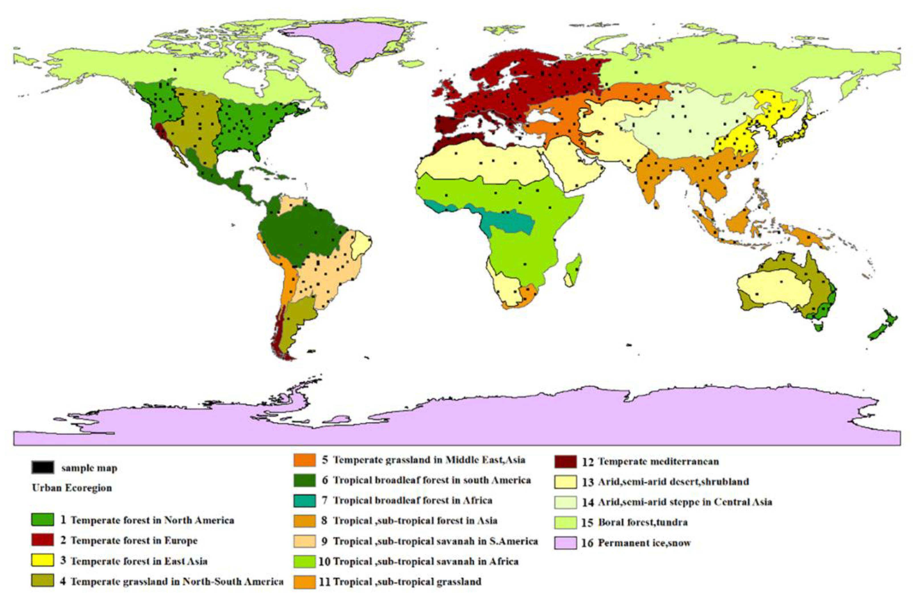
The urban ecoregions proposed by Schneider et al. [33] were used to constitute the spatial strata, and they were sampled independently. This urban ecological stratification was used because the production of the NUACI-based multi-temporal global urban land-cover dataset was based on this stratification. The urban ecological zoning considers the similarities in ecological, cultural, and social factors of urban land use at a global scale, and the global land area is divided into 16 ecological biomes. This stratification method ensures a good spatial distribution of samples around the world. Since the 16th ecological region is perennial ice and snow cover, for which there is no urban land category, this ecological region was not considered in this study. Our study followed the good practices recommended by Olofsson et al. [14].
In this study, urban ecoregions were used as the first-stage sampling strata to enhance the geographic spread of the samples and to produce precise estimates of the user’s accuracy for the rare classes [46]. In order to make the sample maps more evenly distributed in space, each original map (10° × 10°) was divided into (1° × 1°) map sheets, as shown in Figure 7. We then obtained 22,400 map sheets (1° × 1°) covering the entirety of the world. The main difference between the 10° × 10° map sheets and the 1° × 1° map sheets as a sampling unit is that the samples are more scattered and uniform in the global space for the 1° × 1° map sheets and are more representative. These 1° × 1° map sheets formed the primary sampling unit (PSU) and were selected randomly within each urban ecoregion, the purpose of which was to make the sample map sheets more spatially representative. Taking the sample map sheet as the first-stage sampling unit, it was necessary to determine the sample size for the map sheets at a global scale. Generally speaking, as the sample size increases, the standard deviation and the width of the confidence interval of the accuracy and area estimation become smaller, but the increase in the sample size also increases the cost of obtaining samples and the visual interpretation. At this point, the sample’s size should reach an effective balance between accuracy and cost.
According to the principle of probability statistics, a sample size estimation model was established by constraining the relative error between the actual classification error accuracy and the expected classification accuracy error. We calculated the sample size for the map sheets based on the probability sampling statistical model formula [47]. With the 22,400 map sheets as the sampling population, the estimated classification error rate was 20%. The result of the map sheet’s sample size for the multi-period global impervious land-cover data was 378.
The sample’s map sheets were allocated according to the proportion of urban area in each ecological region. The number of sample map sheets in each ecological region is listed in Table 4. Ecological region number 16 covered by perennial ice and snow was not considered in this study as there is no urban area. Because the tropical broadleaf forest in Africa, the boreal forest, and tundra regions cover a small land area, the number of sample map sheets allocated to them is small. The land area of the temperate forest in North America and the temperate forest in Europe accounts for 19% and 15.4% of the total land area of the world. Under the principle of allocation according to the proportion of urban area, the corresponding sample size for these map sheets is 72 and 58, respectively.
Since the number of samples for the map sheets in each ecoregion was determined according to the area percentage, the inclusion probabilities for the map sheet samples in each ecoregion are similar. In each geographic stratum, the PSUs were selected randomly in consideration of the criterion of the stratified random sampling design. Figure 8 shows the result of the distribution of the sample map sheets for the multi-temporal urban land-cover data at a global scale.
We take the three periods of global urban land-cover data as an example. The types of combinations of temporal changes and unchanged of the urban land-cover product were used to obtain eight strata (Table 5). In the temporal domain, the same sampling units were observed at each pixel in the three periods. In the spatial domain, the sampling design is two-stage cluster sampling. This goal is achieved by increasing the sample ratio for the rare change type. There are two types of global urban land cover. For the convenience of presentation, we use 0 to represent non-urban and 1 to represent urban in Table 3. The advantages of such a stratification are as follows: (1) Stratification according to the time series is the basis for evaluating the accuracy of the change and no-change categories between different years; (2) it avoids repeated sampling at the same point. Types 000 and 111 are types that have not changed, indicating that the land cover has been either non-urban or urban and between 2000 and 2010, respectively. Types 001 and 011 are representative of urban expansion and are consistent with the trend of global urban expansion. Types 110 and 100 indicate that the classification label of the urban land changed according to the urban planning policy. These changes are relatively small compared to urban expansion, so they may contain more misclassified information. Type 101 indicates that it was urban land in the year 2000, but it had become non-urban land in 2005 and then became urban land again in the year 2010. This may be representative of the process of demolishing old buildings and restoring new ones. Type 010 indicates that the location was originally non-urban land that has undergone transformation into building land and finally become non-urban land. There can be different reasons for this change to happen, and the demolition of illegal buildings is one of them.
Table 5 shows stratified samplings based on the use of the multi-temporal land-cover change and no-change types to define the strata. The purpose of dividing into eight strata is to improve the accuracy for the rare change types, for which this goal is achieved by increasing the proportion of their samples.
The second stage sampling units refer to the pixels within the first-stage PSUs of each ecological region. The sample units coincide with the resolution of the global urban land-cover product. With a classification error rate of 20%, a confidence level of 95%, and a relative error of 0.05, the number of sample pixels is 6755 based on the probability statistics model for a global scale [47]. The sample size for each ecological region was determined based on the land area of urban to the total area of the global urban land area in the classification map, as shown in Table 6.
3.3. Sample Allocation to the Strata for the Multi-Temporal Global Urban Land-Cover Product
The sample size of 500 was chosen as a trade-off between cost-effectiveness and timeliness. The corresponding error matrix shown in Table 7 was then obtained by visually interpreting the results for these preselected samples. The optimal sample allocation was performed based on the function of the sum of the variance of all strata for the user’s accuracy, producer’s accuracy, and estimated proportion of area. A rule of thumb recommended by Congalton [48] was to use a minimum sample size of 50 for each class in the error matrix. This minimum number should be increased to 75 or 100 if the classification has many classes existing in the classification map or has a large area [48]. The samples allocated to each stratum in the sub-ecoregions are shown in Figure 9.
The implementation of LPM can select a sample from a two-dimensional population. The samples are discretized in space based on LPM [38]. Considering the time consumption, random sampling was used to select the sample points in the unchanged layer (i.e., the 000 stratum) of the temporal data of the three periods, while the LPM method was used to select the sample points in the remaining seven strata.
3.4. Accuracy Estimation
During the accuracy estimation, single accuracy index often leads to an incorrect conclusion. Thus, multiple indicators, such as user’s, producer’s accuracies, etc., are used to evaluate data. In the practical process, in addition to the overall accuracy, accuracy indicators described in Equations (11)–(18) are used for the evaluation.
3.4.1. Single-Date Accuracy Estimates
The accuracy assessment of the single-date global urban area provides important information relative to the quality of the multi-temporal product. The overall accuracy of the global urban area is 97.18% for 2000, 97.11% for 2005, and 96.84% for 2010, with a standard deviation of 0.21%, 0.21%, and 0.22%, respectively (Figure 10a). Overall accuracies of these multi-temporal and single-date urban maps are all more than 95%. This is because the proportion of non-urban areas in many map sheets is very close to 0, and the dominant proportion of non-urban area is classified correctly, resulting in high precision.
The user’s accuracy for the non-urban decreased over time (Figure 10b). However, the user’s accuracy for the urban increased significantly from 58.3 ± 0.82% to 67.27 ± 0.87% over 10 years. These data show that, from 2000 to 2010, the global urbanization area increased, which will increase the probability of the selected samples falling into homogeneous urban plots and will affect the result of its accuracy assessment. There are significant differences in the accuracies between non-urban and urban areas. For non-urban areas, the user’s accuracy at the global scale is above 95%, with the highest accuracy of 98.07 ± 0.3% for 2010 and the lowest accuracy of 97.65 ± 0.3% for 2000. The same trend can be observed in the producer’s accuracy for non-urban and urban areas.
Figure 10b,c also show that the standard deviation of the urban area is greater than that of the non-urban area in the user’s and producer’s accuracies. This is because the urban land area represents a relatively small proportion of the mapped area and is relatively scattered compared to the non-urban land area. The results of the sample interpretation are consistently poor, leading to the large errors. Nevertheless, over the 10 years, non-urban and urban areas were consistently mapped with high accuracy.
3.4.2. Accuracy of the Three Phases of Urban Land Cover for the Change and No-Change Types
The urban land of the three periods was stratified by considering the temporal and spatial characteristics, and then the accuracy was evaluated. At the global scale, 000 refers to the non-urban type, which occupies the largest proportion of the entire area. There may be misclassifications, but this is not related to urban-land errors; thus, this type of error does not affect accuracies. Figure 11 shows that the overall accuracy of above 95% was driven by the large proportion of non-urban area. The user’s accuracy for the non-urban area exceeds 95%. The user’s accuracies for the land-cover change type are generally much lower, at less than 10% for some strata, whereas the producer’s accuracies for the land-cover change type are higher. The user’s accuracies for urban expansion are higher than the user’s accuracies for the land-cover change type. The area proportions of the different types of changes may cause large standard deviations. From Figure 11, the accuracy of the de-urbanization (010, 100, 101, and 110) is very low compared with that of urban gain (001 and 011) since the proportion of de-urbanization is small.
3.4.3. Accuracy for the Change and No-Change Types
The global urban-land area was divided into 15 sub-regions based on the ecological divisions. From Table 8, Table 9 and Table 10, the overall accuracy of the binary change and no-change classification exceeds 90% at the global level. The high overall agreement rate is driven by the large proportion of no-change area. The user’s and producer’s accuracies for no-change are consistently above 90%, whereas the user’s and producer’s accuracies for change are lower and more variable over all sub-regions. The remaining change strata reporting themes have lower user’s accuracies. A partial explanation for the lack of uniformly high user’s accuracies for the reporting themes representing change is evident in the error matrices. The producer’s accuracy of change classification for 2000–2005 (Table 10) is higher than other periods, but it shows high variances. This may be a result of the poor quality of reference data from 2000 to 2005.
At the ecological region scale, the sample size allocated to each region is determined according to the proportion of the urban area’s extent. Therefore, regions 7 and 9 are allocated a small number of samples. The overall accuracies for the different ecological regions are different, and they are all above 90%, with a standard deviation of less than 1%. The highest accuracies are observed in region 15 for the three periods, and the lowest accuracies are found in region 4 (Figure 12). These results demonstrate that the accuracies are different in both the different years and different ecological regions. Therefore, the ecological regions can be considered as heterogeneous entities, and the regional stratified sampling provides a better understanding of the global urban land-cover product [30].
3.4.4. Accuracy of Urban Expansion and No Change
Previous research regarding the accuracy assessment in urban area only considers the stable urban, stable non-urban, and urban gain, i.e., (000, 001, 011, and 111). If we only consider the accuracy calculation of samples from these four layers, samples from other layers will not be included in the calculation. The overall accuracy for the three phases for urban expansion and no change is 96.9 ± 0.3% (Figure 13). From Figure 14a, the overall accuracy for urban land in the three phases significantly improved, compared to the eight-layer change type. The user’s accuracy and producer’s accuracy have the same trend (Figure 14b,c). The OA estimated for the year 2000 is the highest, and it is slightly lower for 2005 and 2010, which is similar to the previous eight-layer evaluation results. The different sampling designs have a direct impact on the accuracy evaluation results for the product. Compared Figure 13 and Figure 14, the user’s accuracies and producer’s accuracies for the four types of strata are improved, compared to those for the eight types (000, 010, 001, 001, 110, 100, 101, and 111). The least accurate stratum is 011.
3.4.5. Accuracy Metrics
Table 11 shows the estimated accuracy metric values at the global scale and their standard deviations for each validation year. The Oe values are higher than the Ce values for the three periods, which is consistent with the negative values of relB, reflecting urban land accuracy underestimation. The year 2010 shows the highest DC of 53% (±5.5%), followed by 2005 at 52% (±5.6%) and 2000 at 48% (±5.7%). The year 2010 achieves the highest accuracy in Ce and DC, while 2000 shows the lowest accuracy in Ce, Oe, and DC. The year 2005 achieves the lowest relB value of −28% (±13.2%). The standard deviation estimates of the four accuracy metrics for 2010 are the lowest. The range of accuracy metrics between the three periods is relatively small. The range of Ce, Oe, and DC is less than 5% for the three periods. The conclusion that can be drawn from these results is that the multi-temporal global urban data have temporal stability.
4. Discussion
In this article, we have proposed a spatio-temporal stratified sampling framework for multi-temporal global urban land-cover data, which is aimed at accurately evaluating single-period data accuracy and also two-period change and no-change type accuracy. In the sampling design, the probability sampling statistical model is used to calculate the sample size of the primary and secondary sampling units. The percentage sampling method has disadvantages, such as strict large batches and loose small batches, and it cannot be applied well for the determination of sample size. Numerous studies have failed to consider how to reasonably determine the sample size when evaluating the accuracy of land-cover products. However, the sample size allocation in the sample design component of accuracy assessment is an important part of improving the accuracy [24]. In the proposed approach, the stratification is determined by global urban ecological regions and spatio-temporal changes, and a two-stage sampling framework is established. During first-stage sampling, a regional stratified random sampling design is used to allocate the samples to the strata according to the proportion of the urban area extent of the global urban land-cover product. Spatio-temporal change stratification provides the technical support for dynamic monitoring of the product. In the second stage, based on the characteristics of the multi-temporal urban land, a method for determining the stratified sample size with an objective function is proposed. Considering the spatial distribution characteristics of urban land cover, the sample pixels are selected by LPM. The proposed new accuracy validation methodology for multi-temporal global urban land-cover data could provide a technical reference for the subsequent accuracy evaluation of similar products.
The accuracy estimations conducted based on a sample of reference data provided valuable information on both the single-date maps and multi-temporal global urban land-cover data for the change and no-change types. When only considering no-change types (000 and 111) and urban expansion (001 and 011) as the strata, it was found that the overall accuracy gradually decreased from 2000 to 2010 (Figure 14a). The accuracy evaluation results for the eight strata considering spatio-temporal changes reached the highest in 2000 and the lowest in 2010 (Figure 10a). An explanation for this is that the proportion of land area occupied by the change strata is small, but it still has an impact on the result of the stratified accuracy assessment. From 2000 to 2010, it was found that the area of urban land had been increasing, and its classification accuracy was lower than that for the non-urban land, which in turn affects the overall accuracy of the product. In future research, a variety of accuracy indicators could be used to evaluate the accuracy of a single type of data product, and it is not limited to the overall accuracy, producer’s accuracy, and user’s accuracy considered in this study. In this paper, the multi-temporal land-cover accuracy assessment experiment uses only three periods of data for validation, and it is expected that more than three periods of data can be used to verify the method in the future. For the method of assigning sample size based on objective function optimization, it is necessary to know the variance of the data in advance. However, in the sampling design stage, this information is not known. It is expected that, in the future, it can be developed with other information of map, such as the area of each stratum in the classification map. Reasonable models for reducing the work intensity caused by pre-sampling will be developed.
There are many factors that influence the accuracy of visual image interpretation: inconsistency in the definition of urban land data [49], misclassification in global urban land data, spatial misalignment between the classification map and reference data, different interpreters labeling the same sample with different reference labels [50], and reference data not being free of errors [51]. Validation procedures need to be improved in future studies.
5. Conclusions
The data quality is a key attribute of multi-temporal global urban land-cover products, and the thematic accuracy is a necessary indicator to implement product quality control. The proposed spatio-temporal stratified sampling method provides an efficient and exact method for validating multi-temporal global urban land-cover products. The two-stage stratification by both global urban ecoregion and spatio-temporal changes provides reasonable samples and, thus, improves the reliability of the accuracy assessment. In addition, the optimal sample size for the stratification is achieved using the initial prejudgment error matrix, and an objective function is constructed by combining the sum of the user’s accuracy variance, producer’s accuracy variance, and estimated area ratio variance of all strata. This approach shows a lower variance in the estimated accuracy than equal allocation and proportional allocation. Furthermore, LPM is used to balance the spatial distribution of the samples, leading to spatially balanced samples and a decrease in sampling variance. From the accuracy assessment of the multi-temporal global urban land-cover product, the main findings are as follows: (1) in the accuracy evaluation of global urban land cover in 2000 and 2010, the overall accuracy of the data slightly decreases as the area of the rare change layer increases; (2) overall accuracies for single dates are more than 95%, but the user’s accuracies need to be improved in future dataset products; (3) the standard deviations of the overall accuracy are less than 1%, indicating that the accuracy evaluation method proposed in this article is effective.
Author Contributions
Conceptualization, Yali Gong, Huan Xie, and Xiaohua Tong; methodology, Yali Gong; software, Yali Gong, Huan Xie, Yanmin Jin, and Xiaohua Tong; validation, Yali Gong; formal analysis, Huan Xie; writing—original draft preparation, Yali Gong; writing—review and editing, Huan Xie and Yanmin Jin; supervision, Xiaohua Tong; project administration, Huan Xie; funding acquisition, Huan Xie and Xiaohua Tong. All authors have read and agreed to the published version of the manuscript.
Funding
This research was funded by the National Natural Science Foundation of China (Project Nos. 41631178 and 41822106), the National Key Research and Development of China (Project No. 2018YFB0505400), the Dawn Scholar of Shanghai (Project No. 18SG22), the State Key Laboratory of Disaster Reduction in Civil Engineering (Project No. SLDRCE19-B-35), and the Fundamental Research Funds for the Central Universities of China.
Institutional Review Board Statement
Not applicable.
Informed Consent Statement
Not applicable.
Data Availability Statement
The dataset are available for downloading at the link: https://www.geosimulation.cn/GlobalUrbanLand.html (8 June 2022).
Acknowledgments
We would like to sincerely thank Xiaoping Liu for providing the multi-temporal global urban land-cover map.
Conflicts of Interest
The authors declare no conflict of interest.
References
- Wang, C.; Zhuo, X.; Li, P.; Chen, N.; Wang, W.; Chen, Z. An Ontology-Based Framework for Integrating Remote Sensing Imagery, Image Products, and In Situ Observations. J. Sens. 2020, 2020, 1–12. [Google Scholar] [CrossRef]
- Mora, B.; Romijn, E.; Herold, M. Monitoring progress towards Sustainable Development Goals—The role of land monitoring. In Proceedings of the 5th GEOSS Science and Technology Stakeholder Workshop—Linking the Sustainable Development Goals to Earth Observations, Models and Capacity Building, Berkeley, CA, USA, 9–10 December 2016. [Google Scholar]
- Stehman, S.V. Sampling designs for accuracy assessment of land cover. Int. J. Remote Sens. 2009, 30, 5243–5272. [Google Scholar] [CrossRef]
- Chen, D.M.; Hui, W. The effect of spatial autocorrelation and class proportion on the accuracy measures from different sampling designs. ISPRS J. Photogramm. Remote Sens. 2009, 64, 140–150. [Google Scholar] [CrossRef]
- Hou, Y.; Burkhard, B.; Müller, F. Uncertainties in landscape analysis and ecosystem service assessment. J. Environ. Manag. 2013, 127, S117–S131. [Google Scholar] [CrossRef]
- Stehman, S.V.; Czaplewski, R.L. Design and Analysis for Thematic Map Accuracy Assessment: Fundamental Principles. Remote Sens. Environ. 1998, 64, 331–344. [Google Scholar] [CrossRef]
- Rwanga, S.S.; Ndambuki, J.M. Accuracy Assessment of Land Use/Land Cover Classification Using Remote Sensing and GIS. Int. J. Geosci. 2017, 8, 611–622. [Google Scholar] [CrossRef]
- Foody, G.M. Sample size determination for image classification accuracy assessment and comparison. Int. J. Remote Sens. 2009, 30, 5273–5291. [Google Scholar] [CrossRef]
- Roy, D.P.; Boschetti, L. Southern Africa Validation of the MODIS, L3JRC, and GlobCarbon Burned-Area Products. IEEE Trans. Geosci. Remote Sens. 2009, 47, 1032–1044. [Google Scholar] [CrossRef]
- Strahler, A.H.; Boschetti, L.; Foody, G.M.; Friedl, M.A.; Hansen, M.C.; Herold, M.; Mayaux, P.; Morisette, J.T.; Stehman, S.V.; Woodcock, C.E. Global Land Cover Validation: Recommendations for Evaluation and Accuracy Assessment of Global Land Cover Maps; European Communities: Luxembourg, 2006. [Google Scholar]
- Stehman, S.V. Statistical Rigor and Practical Utility in Thematic Map Accuracy Assessment. Photogramm. Eng. Remote Sens. 2001, 67, 727–734. [Google Scholar]
- Mcgwire, K.C.; Fisher, P. Spatially Variable Thematic Accuracy: Beyond the Confusion Matrix. In Spatial Uncertainty in Ecology; Springer: New York, NY, USA, 2001. [Google Scholar]
- Foody, G.M. Status of land cover classification accuracy assessment. Remote Sens. Environ. 2002, 80, 185–201. [Google Scholar] [CrossRef]
- Olofsson, P.; Foody, G.M.; Herold, M.; Stehman, S.V.; Woodcock, C.E.; Wulder, M.A. Good practices for estimating area and assessing accuracy of land change. Remote Sens. Environ. 2014, 148, 42–57. [Google Scholar] [CrossRef]
- Chzhen, E. Optimal Rates for Nonparametric F-Score Binary Classification via Post-Processing. Math. Methods Stat. 2020, 29, 87–105. [Google Scholar] [CrossRef]
- Mayaux, P.; Eva, H.; Gallego, J.; Strahler, A.H.; Herold, M.; Agrawal, S.; Naumov, S.; Miranda, E.D.; Bella, C.; Ordoyne, C. Validation of the global land cover 2000 map. IEEE Trans. Geosci. Remote Sens. 2006, 44, 1728–1739. [Google Scholar] [CrossRef]
- Gong, P.; Wang, J.; Yu, L.; Zhao, Y.; Chen, J. Finer resolution observation and monitoring of global land cover: First mapping results with Landsat TM and ETM+ data. Int. J. Remote Sens. 2013, 34, 48. [Google Scholar] [CrossRef]
- Padilla, M.; Stehman, S.V.; Chuvieco, E. Validation of the 2008 MODIS-MCD45 global burned area product using stratified random sampling. Remote Sens. Environ. 2014, 144, 187–196. [Google Scholar] [CrossRef]
- Tsendbazar, N.; Herold, M.; Li, L.; Tarko, A.; de Bruin, S.; Masiliunas, D.; Lesiv, M.; Fritz, S.; Buchhorn, M.; Smets, B.; et al. Towards operational validation of annual global land cover maps. Remote Sens. Environ. 2021, 266, 112686. [Google Scholar] [CrossRef]
- Zhang, X.; Liu, L.Y.; Wu, C.S.; Chen, X.D.; Gao, Y.; Xie, S.; Zhang, B. Development of a global 30 m impervious surface map using multisource and multitemporal remote sensing datasets with the Google Earth Engine platform. Earth Syst. Sci. Data 2020, 12, 1625–1648. [Google Scholar] [CrossRef]
- Guillevic, P.; Göttsche, F.; Nickeson, J.; Hulley, G.; Ghent, D.; Yu, Y.; Trigo, I.; Hook, S.; Sobrino, J.A.; Remedios, J.; et al. Land Surface Temperature Product Validation Best Practice Protocol. Version 1.1. In Good Practices for Satellite-Derived Land Product Validation; Guillevic, P., Göttsche, F., Nickeson, J., Román, M., Eds.; Land Product Validation Subgroup (WGCV/CEOS): College Park, MD, USA, 2018; p. 58. [Google Scholar]
- Woodcock, C.E.; Loveland, T.R.; Herold, M.; Bauer, M.E. Transitioning from change detection to monitoring with remote sensing: A paradigm shift. Remote Sens. Environ. 2020, 238, 111558. [Google Scholar] [CrossRef]
- Liu, M.; Cao, X.; Li, Y.; Chen, X. Method for land cover classification accuracy assessment considering edges. Sci. China 2016, 59, 2318–2327. [Google Scholar] [CrossRef]
- Stehman, S.V. Impact of sample size allocation when using stratified random sampling to estimate accuracy and area of land-cover change. Remote Sens. Lett. 2012, 3, 111–120. [Google Scholar] [CrossRef]
- Cochran, W.G. Sampling Techniques, 3rd ed.; John Wiley & Sons: New York, NY, USA, 1977. [Google Scholar]
- Stehman, S.V.; Foody, G.M. Key issues in rigorous accuracy assessment of land cover products. Remote Sens. Environ. 2019, 231, 111199. [Google Scholar] [CrossRef]
- Liu, S.; Zhao, H.; Du, Q.; Bruzzone, L.; Samat, A.; Tong, X. Novel Cross-Resolution Feature-Level Fusion for Joint Classification of Multispectral and Panchromatic Remote Sensing Images. IEEE Trans. Geosci. Remote Sens. 2021, 60, 1–14. [Google Scholar] [CrossRef]
- Liu, X.; Hu, G.; Chen, Y.; Li, X.; Xu, X.; Li, S.; Pei, F.; Wang, S. High-resolution multi-temporal mapping of global urban land using Landsat images based on the Google Earth Engine Platform. Remote Sens. Environ. 2018, 209, 227–239. [Google Scholar] [CrossRef]
- Stehman, S.V. Estimating area and map accuracy for stratified random sampling when the strata are different from the map classes. Int. J. Remote Sens. 2014, 35, 4923–4939. [Google Scholar] [CrossRef]
- Xie, H.; Tong, X.; Meng, W.; Liang, D.; Wang, Z.; Shi, W. A Multilevel Stratified Spatial Sampling Approach for the Quality Assessment of Remote-Sensing-Derived Products. IEEE J. Sel. Top. Appl. Earth Obs. Remote Sens. 2015, 8, 4699–4713. [Google Scholar] [CrossRef]
- Padilla, M.; Olofsson, P.; Stehman, S.V.; Tansey, K.; Chuvieco, E. Stratification and sample allocation for reference burned area data. Remote Sens. Environ. 2017, 203, 240–255. [Google Scholar] [CrossRef]
- Boschetti, L.; Stehman, S.V.; Roy, D.P. A stratified random sampling design in space and time for regional to global scale burned area product validation. Remote Sens. Environ. 2016, 186, 465–478. [Google Scholar] [CrossRef]
- Schneider, A.; Friedl, M.A.; Potere, D. Mapping global urban areas using MODIS 500-m data: New methods and datasets based on ‘urban ecoregions’. Remote Sens. Environ. 2010, 114, 1733–1746. [Google Scholar] [CrossRef]
- Angel, S.; Sheppard, S.C.; Civco, D.L. The Dynamics of Global Urban Expansion; Transport and Urban Development Department: Washington, DC, USA, 2005.
- Schneider, A.; Friedl, M.A.; McIver, D.K.; Woodcock, C.E. Mapping Urban Areas by Fusing Multiple Sources of Coarse Resolution Remotely Sensed Data. Photogramm. Eng. Remote Sens. 2003, 69, 1377–1386. [Google Scholar] [CrossRef]
- Gamba, P.; Herold, M. Global Mapping of Human Settlement; CRC Press: Boca Raton, FL, USA, 2009. [Google Scholar]
- Olofsson, P.; Stehman, S.V.; Woodcock, C.E.; Sulla-Menashe, D.; Herold, M. A global land-cover validation data set, part I: Fundamental design principles. Int. J. Remote Sens. 2012, 33, 5768–5788. [Google Scholar] [CrossRef]
- Grafström, A.; Lundström, N.L.; Schelin, L. Spatially Balanced Sampling through the Pivotal Method. Biometrics 2012, 68, 514–520. [Google Scholar] [CrossRef] [PubMed]
- Grafström, A.; Matei, A. Spatially Balanced Sampling of Continuous Populations. Scand. J. Stat. 2018, 45, 792–805. [Google Scholar] [CrossRef]
- Olofsson, P.; Arévalo, P.; Espejo, A.B.; Green, C.; Lindquist, E.; McRoberts, R.E.; Sanz, M.J. Mitigating the effects of omission errors on area and area change estimates. Remote Sens. Environ. 2019, 236, 111492. [Google Scholar] [CrossRef]
- Nelson, M.D.; Garner, J.D.; Tavernia, B.G.; Stehman, S.V.; Riemann, R.I.; Lister, A.J.; Perry, C.H. Assessing map accuracy from a suite of site-specific, non-site specific, and spatial distribution approaches. Remote Sens. Environ. 2021, 260, 112442. [Google Scholar] [CrossRef]
- Nowak, D.J.; Greenfield, E.J. Evaluating The National Land Cover Database Tree Canopy and Impervious Cover Estimates Across the Conterminous United States: A Comparison with Photo-Interpreted Estimates. Environ. Manag. 2010, 46, 378–390. [Google Scholar] [CrossRef]
- Wickham, J.; Stehman, S.V.; Gass, L.; Dewitz, J.A.; Sorenson, D.G.; Granneman, B.J.; Poss, R.V.; Baer, L.A. Thematic accuracy assessment of the 2011 National Land Cover Database (NLCD). Remote Sens. Environ. 2017, 191, 328–341. [Google Scholar] [CrossRef]
- Franquesa, M.; Lizundia-Loiola, J.; Stehman, S.V.; Chuvieco, E. Using long temporal reference units to assess the spatial accuracy of global satellite-derived burned area products. Remote Sens. Environ. 2022, 269, 112823. [Google Scholar] [CrossRef]
- Forbes, A.D. Classification-algorithm evaluation: Five performance measures based on confusion matrices. J. Clin. Monit. 1995, 11, 189–206. [Google Scholar] [CrossRef]
- Stehman, S.V.; Wickham, J.; Smith, J.H.; Yang, L. Thematic accuracy of the 1992 National Land-Cover Data for the eastern United States: Statistical methodology and regional results. Remote. Sens. Environ. 2003, 86, 500–516. [Google Scholar] [CrossRef]
- Tong, X.; Wang, Z.; Xie, H.; Liang, D.; Jiang, Z.; Li, J.; Li, J. Designing a two-rank acceptance sampling plan for quality inspection of geospatial data products. Comput. Geosci. 2011, 37, 1570–1583. [Google Scholar] [CrossRef]
- Congalton, R. Putting the Map Back in Map Accuracy Assessment. In Remote Sensing and GIS Accuracy Assessment; CRC Press: Boca Raton, FL, USA, 2004. [Google Scholar]
- Congalton, R.G.; Gu, J.; Yadav, K.; Thenkabail, P.; Ozdogan, M. Global Land Cover Mapping: A Review and Uncertainty Analysis. Remote Sens. 2014, 6, 12070–12093. [Google Scholar] [CrossRef]
- Xing, D.; Stehman, S.V.; Foody, G.M.; Pengra, B.W. Comparison of Simple Averaging and Latent Class Modeling to Estimate the Area of Land Cover in the Presence of Reference Data Variability. Land 2021, 10, 35. [Google Scholar] [CrossRef]
- Foody, G.M. Assessing the accuracy of land cover change with imperfect ground reference data. Remote Sens. Environ. 2010, 114, 2271–2285. [Google Scholar] [CrossRef]
Figure 1.
SH data set. (a) Classification map. (b) Reference map.

Figure 2.
Data distribution of global urban land cover.

Figure 3.
Example of the combination of the land-cover types in three different dates.

Figure 4.
Comparison between SRS and LPM. (a) SRS. (b) LPM.

Figure 5.
Sample allocation based on the three different methods.

Figure 6.
Comparison of the accuracy absolute bias between the three distribution methods and ground truth (the blue bars show the bias between the EA accuracy and ground truth. The green bars show the bias between the PA accuracy and ground truth. The yellow bars show the bias between the OPA accuracy and ground truth).

Figure 7.
10° × 10° map sheets divided into 1° × 1° map sheets.

Figure 8.
The spatial distribution of the sample map sheets for the global multi-temporal urban land-cover data. The black squares represent the 1° × 1° PSUs. The panels in different colors represent the different urban ecological regions. The map of global urban land cover shows 16 geographic strata.

Figure 9.
The sample allocation for each stratum in the sub-ecoregions (1–15 denote the index of the urban ecoregions corresponding to Figure 8).
Figure 9.
The sample allocation for each stratum in the sub-ecoregions (1–15 denote the index of the urban ecoregions corresponding to Figure 8).

Figure 10.
Accuracy estimation for the multi-temporal global urban land-cover product in single dates. (a) OA, (b) UA, and (c) PA.
Figure 10.
Accuracy estimation for the multi-temporal global urban land-cover product in single dates. (a) OA, (b) UA, and (c) PA.

Figure 11.
Accuracy estimation of the three phases of urban land for the change and no-change types (000–111 denote the urban land change and no-change types corresponding to Table 5). OA = 96.1 ± 0.25%.
Figure 11.
Accuracy estimation of the three phases of urban land for the change and no-change types (000–111 denote the urban land change and no-change types corresponding to Table 5). OA = 96.1 ± 0.25%.

Figure 12.
The OA of the different ecological regions for urban land from 2000 to 2010 at a 95% confidence level (1–16 denote the urban ecoregions corresponding to Figure 7).
Figure 12.
The OA of the different ecological regions for urban land from 2000 to 2010 at a 95% confidence level (1–16 denote the urban ecoregions corresponding to Figure 7).

Figure 13.
Accuracy estimation for the global three-phase urban land cover for the change and no-change type (000–111 denote the three-phase urban land change and no-change types corresponding to Table 5). OA = 96.9 ± 0.3%.
Figure 13.
Accuracy estimation for the global three-phase urban land cover for the change and no-change type (000–111 denote the three-phase urban land change and no-change types corresponding to Table 5). OA = 96.9 ± 0.3%.

Figure 14.
Accuracy estimation of urban expansion and no change in the three periods. (a) OA, (b) UA, (c) PA.
Figure 14.
Accuracy estimation of urban expansion and no change in the three periods. (a) OA, (b) UA, (c) PA.


Table 1.
Global urban land-cover data legends for the classification labels.
| Class | Description |
|---|---|
| Urban | Impervious surface, i.e., artificial cover and structures such as pavement, concrete, brick, stone, and other man-made impenetrable land-cover types |
| Non-urban | Other categories except urban land, e.g., water, barren, forest, grassland, shrubland, cropland, wetland, and perennial ice |
Table 2.
Population error matrix for land-cover data with M classes.
| Reference Class | ||||||||
|---|---|---|---|---|---|---|---|---|
| Map class | 1 | 2 | … | k | … | M | Total | |
| 1 | p11 | p12 | … | p1k | … | p1M | p1+ | |
| 2 | p21 | p22 | … | p2k | … | p2M | p2+ | |
| … | … | … | … | … | … | … | … | |
| k | pk1 | pk2 | … | pkk | … | pkM | pk+ | |
| … | … | … | … | … | … | … | … | |
| M | pM1 | pM2 | pMk | … | pMM | pM+ | ||
| Total | p+1 | p+2 | … | p+k | … | p+M | 1 | |
Table 3.
The initial prejudgment error matrix.
| Map | 1 | 2 | 3 | 4 | 5 |
|---|---|---|---|---|---|
| 1 | 0.4717 | 0.0067 | 0 | 0 | 0 |
| 2 | 0.0213 | 0.2057 | 0 | 0 | 0 |
| 3 | 0 | 0 | 0.1979 | 0 | 0 |
| 4 | 0.0017 | 0.0017 | 0 | 0.0297 | 0 |
| 5 | 0.0001 | 0.0001 | 0 | 0 | 0.0631 |
Table 4.
The sample sizes for the map sheets of the global urban land-cover product in each urban ecoregion (1–16 denote the index of the urban ecoregions corresponding to Figure 7).
Table 4.
The sample sizes for the map sheets of the global urban land-cover product in each urban ecoregion (1–16 denote the index of the urban ecoregions corresponding to Figure 7).
| Urban Ecoregion | Area Proportion (%) | Sample Size for Map Sheets | Urban Ecoregion | Area Proportion (%) | Sample Size for Map Sheets |
|---|---|---|---|---|---|
| 1 | 19 | 72 | 9 | 7.2 | 27 |
| 2 | 15.4 | 58 | 10 | 2.8 | 11 |
| 3 | 8.9 | 34 | 11 | 1.9 | 7 |
| 4 | 5.2 | 20 | 12 | 6.8 | 26 |
| 5 | 5.7 | 22 | 13 | 5.9 | 22 |
| 6 | 3.2 | 12 | 14 | 3.9 | 15 |
| 7 | 0.9 | 3 | 15 | 0.9 | 3 |
| 8 | 12.3 | 46 | 16 | NA | 0 |
Table 5.
The stratification design based on the multi-temporal land-cover change and no-change types, where 1 refers to urban land and 0 refers to non-urban.
Table 5.
The stratification design based on the multi-temporal land-cover change and no-change types, where 1 refers to urban land and 0 refers to non-urban.
| Stratum No. | Stratum Code (2000–2005–2010) | Description |
|---|---|---|
| 1 | 001 | non-urban–non-urban–urban |
| 2 | 010 | non-urban–urban–non-urban |
| 3 | 011 | non-urban–urban–urban |
| 4 | 100 | urban–non-urban–non-urban |
| 5 | 101 | urban–non-urban–urban |
| 6 | 110 | urban–urban–non-urban |
| 7 | 111 | urban–urban–urban |
| 8 | 000 | non-urban–non-urban–non-urban |
Table 6.
Sample size for the pixels in each ecological region (1–15 denote the index of the urban ecoregions corresponding to Figure 8).
Table 6.
Sample size for the pixels in each ecological region (1–15 denote the index of the urban ecoregions corresponding to Figure 8).
| Ecoregion | The Number of Pixels | Sample Size | Ecoregion | The Number of Pixels | Sample Size |
|---|---|---|---|---|---|
| 1 | 1,001,921,757 | 1181 | 9 | 374,695,959 | 449 |
| 2 | 805,784,274 | 948 | 10 | 152,369,949 | 180 |
| 3 | 473,804,814 | 613 | 11 | 97,261,599 | 116 |
| 4 | 278,150,583 | 327 | 12 | 361,900,431 | 428 |
| 5 | 306,035,037 | 362 | 13 | 305,830,932 | 366 |
| 6 | 166,093,227 | 196 | 14 | 208,762,305 | 247 |
| 7 | 41,470,425 | 53 | 15 | 41,604,021 | 50 |
| 8 | 638,006,253 | 752 | 1–15 | 5,253,691,566 | 6268 |
Table 7.
The initial prediction error matrix (000–111 denote the three-phase urban land change and no-change types corresponding to Table 5).
Table 7.
The initial prediction error matrix (000–111 denote the three-phase urban land change and no-change types corresponding to Table 5).
| Reference | |||||||||
|---|---|---|---|---|---|---|---|---|---|
| Map | 1(000) | 2(001) | 3(010) | 4(011) | 5(100) | 6(101) | 7(110) | 8(111) | Total |
| 1(000) | 92 | 1 | 0 | 2 | 0 | 0 | 0 | 5 | 100 |
| 2(001) | 10 | 21 | 0 | 1 | 0 | 0 | 0 | 18 | 50 |
| 3(010) | 30 | 4 | 6 | 7 | 0 | 0 | 0 | 3 | 50 |
| 4(011) | 3 | 8 | 3 | 22 | 0 | 1 | 1 | 12 | 50 |
| 5(100) | 30 | 1 | 0 | 2 | 7 | 1 | 0 | 9 | 50 |
| 6(101) | 10 | 16 | 1 | 3 | 5 | 4 | 0 | 11 | 50 |
| 7(110) | 13 | 1 | 4 | 2 | 2 | 2 | 14 | 12 | 50 |
| 8(111) | 7 | 2 | 0 | 6 | 0 | 0 | 1 | 84 | 100 |
| Total | 195 | 54 | 14 | 45 | 14 | 8 | 16 | 154 | 500 |
Table 8.
Error matrix for the binary change and no-change classification for 2005–2010. The values in parentheses are standard deviations. OA = 98.78 ± 0.14%.
Table 8.
Error matrix for the binary change and no-change classification for 2005–2010. The values in parentheses are standard deviations. OA = 98.78 ± 0.14%.
| Reference | ||||
|---|---|---|---|---|
| Map | No Change | Change | Total | Users |
| No change | 0.9862 | 0.0047 | 0.9909 | 99.52 (0.13) |
| Change | 0.0075 | 0.0016 | 0.0091 | 17.36 (0.66) |
| Total | 0.9937 | 0.0063 | ||
| Prod | 99.25 (0.02) | 24.98 (4.04) | ||
Table 9.
Error matrix for the binary change and no-change classification for 2000–2010. The values in parentheses are standard deviations. OA = 98.79% ± 0.14%.
Table 9.
Error matrix for the binary change and no-change classification for 2000–2010. The values in parentheses are standard deviations. OA = 98.79% ± 0.14%.
| Reference | ||||
|---|---|---|---|---|
| Map | No Change | Change | Total | Users |
| No change | 0.9845 | 0.0050 | 0.9895 | 99.49 (0.13) |
| Change | 0.0070 | 0.0035 | 0.0105 | 33.27 (0.83) |
| Total | 0.9915 | 0.0085 | ||
| Prod | 99.30 (0.02) | 40.6 (4.86) | ||
Table 10.
Error matrix for the binary change and no-change classification for 2000–2005. The values in parentheses are standard deviations. OA = 99.23 ± 0.11%.
Table 10.
Error matrix for the binary change and no-change classification for 2000–2005. The values in parentheses are standard deviations. OA = 99.23 ± 0.11%.
| Reference | ||||
|---|---|---|---|---|
| Map | No Change | Change | Total | Users |
| No change | 0.9905 | 0.0007 | 0.9912 | 99.93 (0.05) |
| Change | 0.0069 | 0.0018 | 0.0087 | 20.73 (0.69) |
| Total | 0.9974 | 0.0025 | ||
| Prod | 99.30 (0.01) | 71.32 (10.36) | ||
Table 11.
Estimated accuracy (expressed as %) for the global urban product in each validation year. The standard deviation is shown in parenthesis.
Table 11.
Estimated accuracy (expressed as %) for the global urban product in each validation year. The standard deviation is shown in parenthesis.
| Year | Ce | Oe | Dc | relB |
|---|---|---|---|---|
| 2000 | 42 (1.6) | 59 (8.1) | 48 (5.7) | −30 (14) |
| 2005 | 38 (1.5) | 55 (8.2) | 52 (5.6) | −28 (13.2) |
| 2010 | 33 (1.4) | 56 (7.4) | 53 (5.5) | −35 (11) |
Publisher’s Note: MDPI stays neutral with regard to jurisdictional claims in published maps and institutional affiliations. |
© 2022 by the authors. Licensee MDPI, Basel, Switzerland. This article is an open access article distributed under the terms and conditions of the Creative Commons Attribution (CC BY) license (https://creativecommons.org/licenses/by/4.0/).
Share and Cite
MDPI and ACS Style
Gong, Y.; Xie, H.; Jin, Y.; Tong, X. Assessing Multi-Temporal Global Urban Land-Cover Products Using Spatio-Temporal Stratified Sampling. ISPRS Int. J. Geo-Inf. 2022, 11, 451. https://doi.org/10.3390/ijgi11080451
AMA Style
Gong Y, Xie H, Jin Y, Tong X. Assessing Multi-Temporal Global Urban Land-Cover Products Using Spatio-Temporal Stratified Sampling. ISPRS International Journal of Geo-Information. 2022; 11(8):451. https://doi.org/10.3390/ijgi11080451
Chicago/Turabian StyleGong, Yali, Huan Xie, Yanmin Jin, and Xiaohua Tong. 2022. "Assessing Multi-Temporal Global Urban Land-Cover Products Using Spatio-Temporal Stratified Sampling" ISPRS International Journal of Geo-Information 11, no. 8: 451. https://doi.org/10.3390/ijgi11080451
Note that from the first issue of 2016, this journal uses article numbers instead of page numbers. See further details here.