Classification of Hydrological Relevant Parameters by Soil Hydraulic Behaviour

Institute of Technology Leichtweiß-Institute for Hydraulic Engineering and Water Resources, Department of Hydrology, Water Resources Management and Water Protection, University of Braunschweig, Beethovenstr. 51a, Braunschweig D-38106, Germany
*
Author to whom correspondence should be addressed.
Geosciences 2019, 9(5), 206; https://doi.org/10.3390/geosciences9050206
Submission received: 1 March 2019
/
Revised: 26 April 2019
/
Accepted: 28 April 2019
/
Published: 8 May 2019
Abstract
:Soil water simulations on hydrological meso- or macroscale require parameters that describe the physical characteristics of the soil. At these scales, information regarding soil properties is mostly only available on very coarse spatial resolutions with texture based soil characterisations, where it is difficult to select representative soil hydraulic parameters. We improved the parameter estimation by introducing a new soil classification system, which is based on soil hydraulic behaviour in order to realistically reproduce the soil water interaction within meso-scaled hydrological models. The time series of soil water flux were simulated based on one million different parameterisations, which were then utilised for similarity analyses while applying the k-means clustering. The resulting classes show a different pattern when compared to the United States Department of Agriculture (USDA) texture based classes. Representative time series of water flux representative of the new classes were compared to time series of the USDA texture classification. The new classes show remarkably lower uncertainties. The bandwidth of the time series within a class is orders of magnitudes higher for the USDA system when compared to the new system. The evaluation of similarity of the simulated water flux time series within one and the same class were also clearly better for the new system.
1. Introduction
State of the art hydrological applications require a spatially distributed model with a physically based process description. Aboveground river systems and small-scale characteristics of soil or vegetation affect the spatial resolution. These different variables have to be parameterised in reconciliation with available measurement or observational data. In this context, a challenge in hydrological process modelling is to minimise the discrepancy between the model’s resolution and the data scale. Data availability mostly “prescribes” the smallest calculation unit of a model. Hydrological processes, which are dominant at spatial scales that are larger than the smallest calculation unit of the model, are assumed to be directly described by the model. Small scale processes below the smallest spatial calculation unit are assumed to be indirectly described by the model, e.g., by calibration [1,2].
The main objective of the study at hand is to improve the parameter estimation for meso-scale hydrological models in order to realistically reproduce the soil water interaction. Soil water movement and storage can be particularly sensitive to many hydrological variables, and therefore affect various simulation outputs, like runoff, infiltration, groundwater recharge, and actual evapotranspiration. Especially, the water content in the soil near the surface has a decisive influence on runoff generation [3,4,5]. Soil water simulations on the catchment scale require parameters, which describe the physical characteristics of the soil. Hence, the soil hydraulic parameterisation is an essential aspect in any hydrological model application [6]. At the hydrological meso- or macroscale, information regarding soil properties is mostly only available on very coarse spatial resolutions, e.g., soil maps with scale of 1:50000. Commonly, such maps provide simplified soil characterisations that are based on their texture [7]. Soil texture is defined as the particle size composition expressed as relative fractions of sand, silt, and clay. The advantage of this classification is that the measurability of the particle sizes is easy and affordable. Furthermore, a regionalisation of these (point) measurements is feasible. The most established classification is the system of the United States Department of Agriculture (USDA), which initially was elaborated by [8]. The general assumption of any soil classification is that the “soils” within each class are as similar as possible to each other. The similarity has to be objectively assessed, e.g., as it is done by texture in the USDA system. This classification is reasonable regarding particle size. The pioneering studies of [9] and [10] questioned the physical reliability of this system concerning soil hydraulic parameters. [9] investigated, whether a classification that was based on hydraulic characteristics—and not texture as single criterion—led to different patterns within the texture triangle. They selected properties, such as field capacity, wilting point, porosity, saturated hydraulic conductivity, drainability, and capillary pressure at field capacity. The classification results were different to the USDA classification for soils with low sand content. [9] argued that, from a soil hydraulic point of view, a classification that is based on texture does not work well for soils with a considerable high impact from capillary forces. However, the question of parameterisation of large scale hydrological soil models in a way that considers hydraulic behaviour still remains. [10] applied a physically based soil-atmosphere-transfer model [11] with more than 5000 realisations of synthetic soil hydraulic parameterisations, according to the Brooks and Corey function [12]. The simulation results (water balance components), as well as the associated soil hydraulic parameters, were used for cluster analyses. The results showed similarities between clusters that were based on soil hydraulic parameters and texture based classification, but different patterns for classification based on simulated water balance. [10] argued that soil texture classification with regard to hydrological aspects could improve the applicability of classified soil data on large scales. [13] applied the HYDRUS one-dimensional (1D) model [14], with 1326 realisations of synthetic parameterisations according to the van Genuchten function [15]. Different kinds of cluster analyses were conducted and various variants of the model were used. One cluster analyse was based on saturated hydraulic conductivity. The others were based on the comparison of water storage prior to and after the simulation. The first model variant only accounted for infiltration, the second variant for drainage, and the third one for both. The cluster patterns differed from USDA texture based pattern, in addition, they also differed from each other.
The above-mentioned studies indicate that a texture based classification of soils may not be the optimal solution with respect to hydrological modelling. The alternative, which could be a classification that is based on soil hydraulic parameters or soil water model results, on the other hand, has not been sufficiently addressed so far and the water balance or the change of water storage is a very general input variable for the clustering.
In the study at hand, simulated time series of soil water flux in high temporal resolutions are utilised as the input in the creation of classes, based on soil hydraulic behaviour, since the flux controls the subsurface discharge components as well as the groundwater recharge. Furthermore, the considered number of samples for the hydraulic parameterisation is much larger than in previous research. We applied more than one-million simulations that are based on Richards equation [16] for two different atmospheric boundary conditions. The k-means clustering [17,18] was applied as a classification algorithm with the water flux as the classification variable. The time series of water flux representative of the new classes were compared to time series representative for USDA texture classification.
2. Materials and Methods
2.1. General Procedure
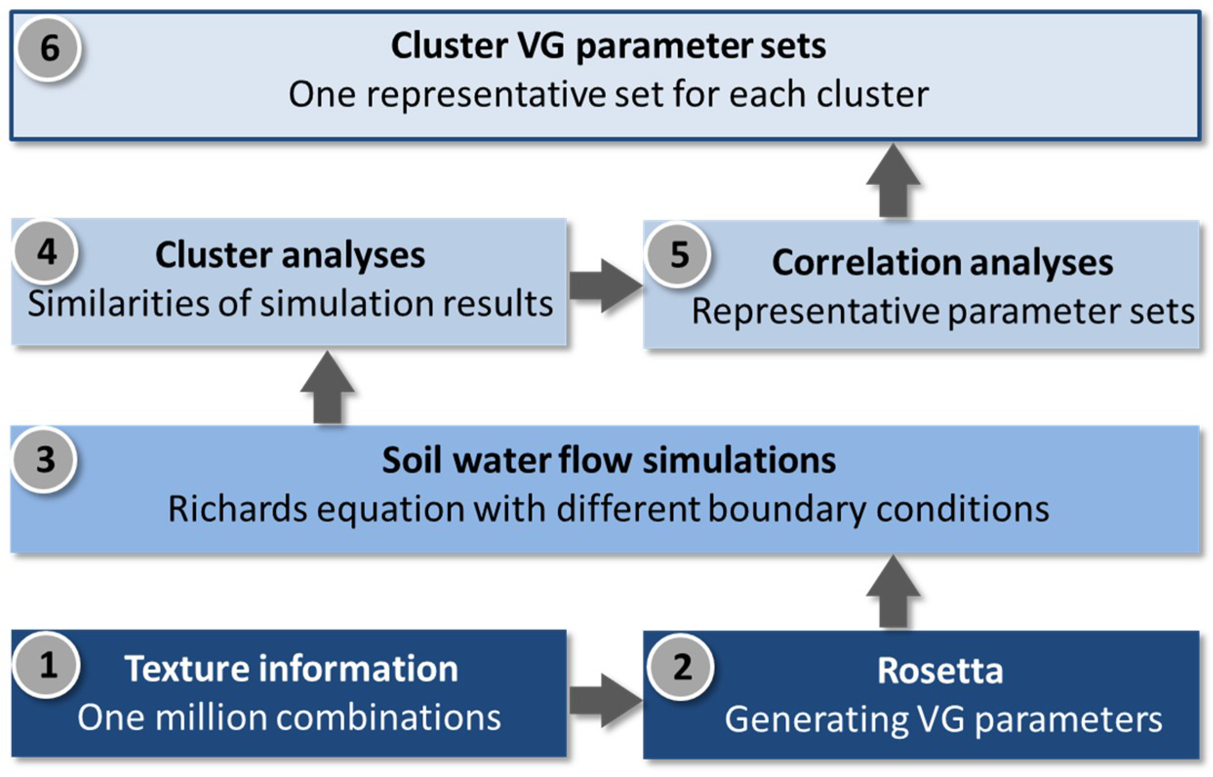
Figure 1 visualizes the general approach of this study. At first, we generated 106 equally distributed numbers with the condition that the sum of (always three) numbers has to be one. The resulting three fractions were assigned to sand, silt, and clay content, while keeping the total sum at of these fractions at 100%. Subsequently, these particle triplets were passed to the software ROSETTA, (free of charge software, which is based on a hierarchical neural network, see e.g., [19,20,21]), by which the van Genuchten [15] parameters (VGP) for each of the triplets were created. These VGP were used to perform soil water simulations on the basis of the Richards equation [16]. 106 of these simulations were numerically solved with an impulse input as the upper boundary condition. A more complex dynamic upper boundary condition was applied to an additional simulation of a subset with 105 triplets. This was done in order to generate different unsaturated conditions throughout the simulation period. The deepness of the domains was assigned to 200 cm, respectively, 400 cm in order to have no influence of the lower boundary condition. We set this condition to constant pressure head, but also applied the free drainage condition with the same classification results. The outputs of these simulations were water fluxes at different soil depths. These time series were used to perform a classification with the help of a k-means cluster algorithm [17,18]. Each of the 106 triplets was thereby assigned to a soil cluster. The advantage of this procedure is that the classification is based on the hydraulic behaviour of the soils, which is an important characteristic for any hydrological model application.
2.2. Soil Hydraulic Models
The model of van Genuchten [15] is the most established way to describe the relation between water content and pressure head in soils.
| with: | |||
| Soil water saturation | (m³∙m−3) | ||
| Soil water pressure head | (m) | ||
| Van Genuchten parameter | (m−1) | ||
| Van Genuchten parameter | (-) | ||
| Van Genuchten parameter | (-) |
The soil water saturation is the standardised form of the volumetric water content with the range from zero (pore volume filled with air) to one (pore volume filled with water), see e.g., [22].
| with: | |||
| Volumetric water content | (m³∙m−3) | ||
| Residual volumetric water content | (m³∙m−3) | ||
| Saturated volumetric water content | (m³∙m−3) |
The studies of [23] and [24] showed the influence of the shape parameters on the simulated water retention curve in detail. The parameter m is commonly approximated to 1–1/n, which reduces the flexibility of the model, but enables a closed form expression of the unsaturated hydraulic conductivity by combining equation (1) with the pore size model of [25].
| with: | |||
| Unsaturated hydraulic conductivity | (m∙s−1) | ||
| Saturated hydraulic conductivity | (m∙s−1) | ||
| Empirical parameter (mostly l = 0.5) | (-) |
Richard’s equation can simulate soil water movement under transient flow conditions [16]. For 1D and without sources and sinks, it can be written, as follows [22]:
| with: | |||
| Time | (s) | ||
| Flow length, positive upward | (m) |
This second order partial differential equation can be solved numerically.
2.3. Soil Hydraulic Parameters
A short algorithm was developed to randomly generate triplets of texture within a percentage range of 0–100 each with the constraint that the sum is always 100 percent. The triplets contain percentage fractions of sand, silt, and clay. In this way, 106 artificial samples of possible compositions of texture fractions were obtained. The large number of generated samples was empirically determined in order to obtain a representative population for the statistical analyses.
The ROSETTA software was used to estimate values of the van Genuchten parameters Θr, Θs, α, and n, as well as Ks for each sample. ROSETTA is established in soil physical disciplines and it is used in several studies, see e.g., [7,26,27]. It is based on neural network analyses and was calibrated by means of a large database comprised of 2134 soil samples that consists of more than 20,000 measured pairs of Θ and h in total. 1306 soil samples were available for the saturated hydraulic conductivity. A total of 235 samples also contained data for the unsaturated hydraulic conductivity function K(Θ), including more than 4000 data points [28]. The database UNSODA [20,21] significantly contributes to these data points.
2.4. Simulation of Soil Water Movement
The partial differential equations for the description of the soil water movement were numerically solved. The numerical solver is based on the work of [29]. The algorithm solves the initial-boundary value problems for systems of parabolic and elliptic PDEs (partial differential equation) in one space variable and time. The solver was applied one million times on the equation of Richards [16], where the VGP of the different texture triplets were used for parameterisation. We additionally applied the HYDRUS-1D model [14] by controlling the “H1D_CALC.EXE” with MATLAB and modifying the “SELECTOR.IN” file, which holds the soil hydraulic parameters to double check the numerical solution.
Two variants of upper boundary conditions were considered:
- An “impulse” boundary condition (IBC), which provides 0.1 cm/d flux for 30 days.
- A “dynamic” boundary condition (DBC), which is a time series of measured precipitation in cm/h, with a length 89 days and a total amount of precipitation of approx. 14 cm.
The total depth “L” of the simulated domain was 200 cm (with IBC) and 400 cm (with DBC), respectively. The initial condition of the hydraulic potential was set to be equal in every depth. Hence, the matrix potential is compensating the gravitational potential and there is no initial water movement. That is why we set the matrix potential at the bottom to—L cm. With these settings, 106 simulation runs were conducted with the IBC, and another 105 simulations were conducted with the DBC. The results comprised time series of water flux for several depths.
2.5. Soil Classification by Soil Hydraulic Response
The results of the soil water simulations were used to group the different soil hydraulic responses and thus to create a new soil hydraulic classification system for soils. We used the water fluxes at a depth of 40 cm for the 106 (IBC), respectively, 105 (DBC) simulations. In this way, the hydraulic response of every possible combination in the texture triangle is considered in the classification. The time series of the simulations with IBC and DBC were individually treated.
The k-means clustering was applied as the classification algorithm. This algorithm is based on the work of [17] and [18]. In contrast to the often recommended dynamic time warping method, the k-means has the advantage of being mass conservative, which is essential in soil hydraulics. The input data for the cluster algorithm were the 106 and 105 time series and the objective was set to maximum correlation within the clusters.
2.6. Identification of Representative Parameter Sets
The number of clusters had to be predefined. We tested the influence of this number by repeating the algorithm 38 times with a number of clusters from 3 to 40 and compared the results to the empirical rule after [30]. Further, correlation analyses were conducted to figure out the optimal number of clusters. Several objective functions (quality criteria) were calculated for every single time series of water flux when compared to the arithmetic mean time series of all other time series within one class, since every class will hold many thousand time series of water flux. In a loop over the number of class members, the criteria were calculated between every single time series and the mean time series of the corresponding class. The following objective functions were used (see e.g., [31,32,33,34]).
| with: | |||
| Pearson correlation coefficient | (-) | ||
| Root mean squared error | (m∙s−1) | ||
| Model efficiency | (-) | ||
| Index of agreement | (-) | ||
| Shift of position between peak values | (s) | ||
| Entries of test time series | (m∙s−1) | ||
| Average value of test time series | (m∙s−1) | ||
| Entries of arithmetic mean time series | (m∙s−1) | ||
| Average value of arithmetic mean time series | (m∙s−1) | ||
| Length of time series | (-) |
RMSE has the same unit as the input time series (water flux) and the optimal RMSE is zero. The other quality criteria are dimensionless and have their optimum at a value of one (R also at −1). The range of R is from −1 to 1, Nash has a range from −∞ to 1 and d from 0 to 1.
The average value of each objective function was calculated for each number of clusters. The optimal number of clusters was then determined at a point, at which the improvement of objective functions values was marginal (elbow criterion). We compared the results with the Sturges equation [30], which approximates the ideal number of classes in the dependency of the number of samples.
| with: | |||
| Ideal number of classes | (-) | ||
| Number of samples | (-) |
One representative sample for each cluster had to be identified after the ideal number of clusters had been determined. Every single time series of water flux was compared to the arithmetic mean of the time series. The time series with the highest correlation was identified as the most representative for the associated cluster.
3. Results
3.1. Number of Clusters
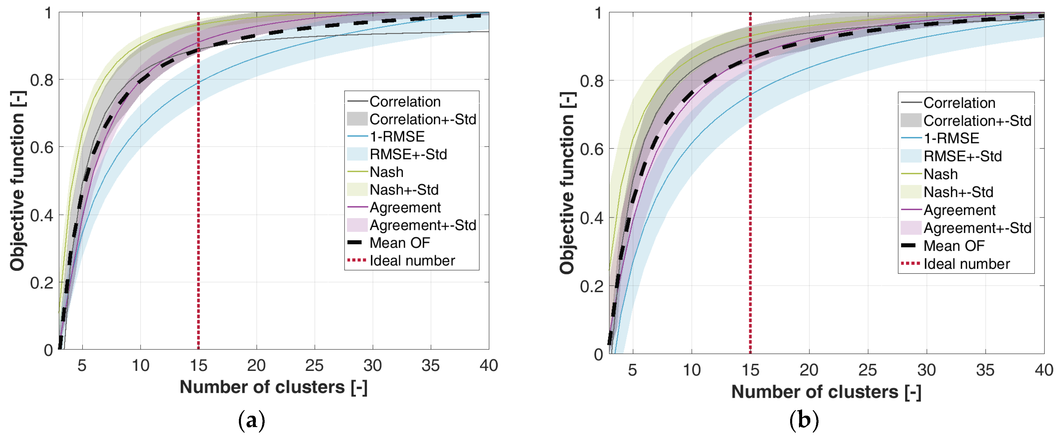
Figure 2 shows the values of the objective functions in the dependence of the number of clusters that were used for the cluster analyses. The general pattern of the analysis that is based on IBC (Figure 2a) and DBC (Figure 2b) is very similar to each other. In addition, the different objective functions show comparable courses after standardisation to a range from zero (no agreement) to one (perfect agreement). An arithmetic mean curve (dashed, bold line) was calculated that was based on all objective functions. The agreement of similarity within the clusters rapidly increases with an ascending numbers of clusters. At approx. a number of nine clusters, the gradients of the objective functions start to decrease and, after 15 clusters, the objective functions hardly improve. Following this visual interpretation (elbow criterion), the ideal number of clusters was set to a value of 15. This corresponds quite well to the ideal number after the Sturges rule [30]. With a sample size of 105 (DBC), a class number of 17–18 was calculated. A sample size of 106 (IBC) was yielded in 21 classes. We preferred the ideal number of 15 clusters to be more convenient although these numbers are slightly higher than the number that was obtained by the elbow criterion.
3.2. Classification Results
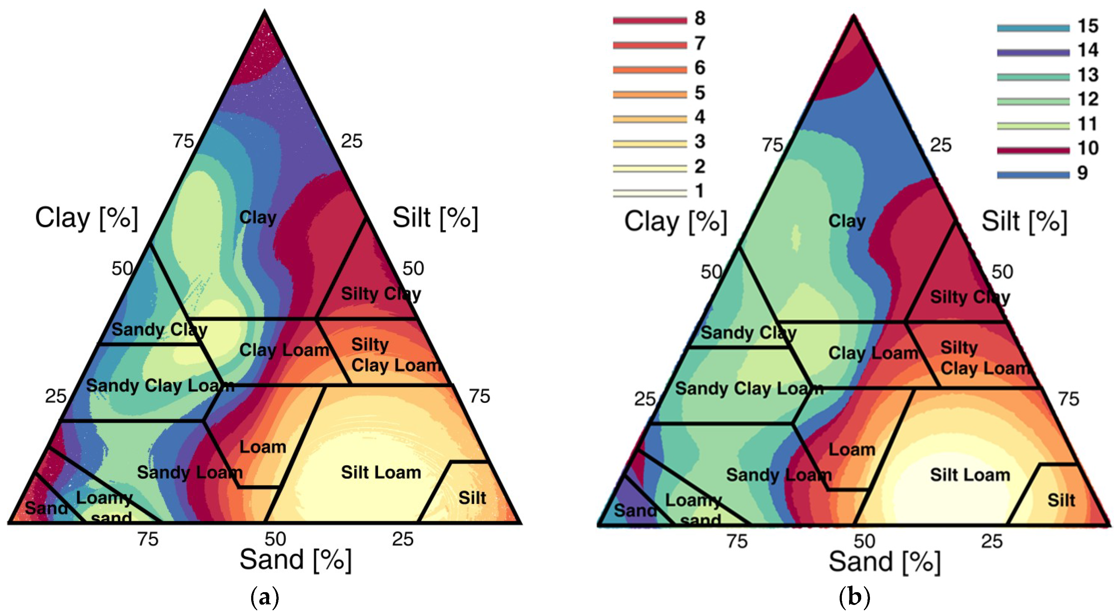
The results of the classification into 15 classes that are based on hydraulic response are visualised within the texture triangle (Figure 3). The 15 new classes are illustrated with different colours. This allows for a direct comparison to the USDA texture based classification, which is divided into 12 classes. The resulting triangle on the left hand side of Figure 3 is based on IBC and the triangle on the right hand side is based on DBC. Both the IBC and DBC classification results show a clear structured pattern. Secondly, these classifications are very similar to each other. On the other hand, both of the classifications based on the hydraulic response are different when compared to the texture based classification. At the bottom of Figure 3, the representative time series of water flux for the 15 classes are shown with the same designated colour as in the triangles. Time series that are based on IBC are presented on the left hand side and time series based on DBC are presented on the right. As anticipated, the 15 different time series clearly differ from each other regarding the general shape, the peak(s), and the time that is taken to attain the peak(s).
We focus on the DBC results hereafter, since the classification results of IBC and DBC show a high agreement to each other and DBC is based on more input information, resulting in a less frayed pattern. Table 1 lists the representative VGP.
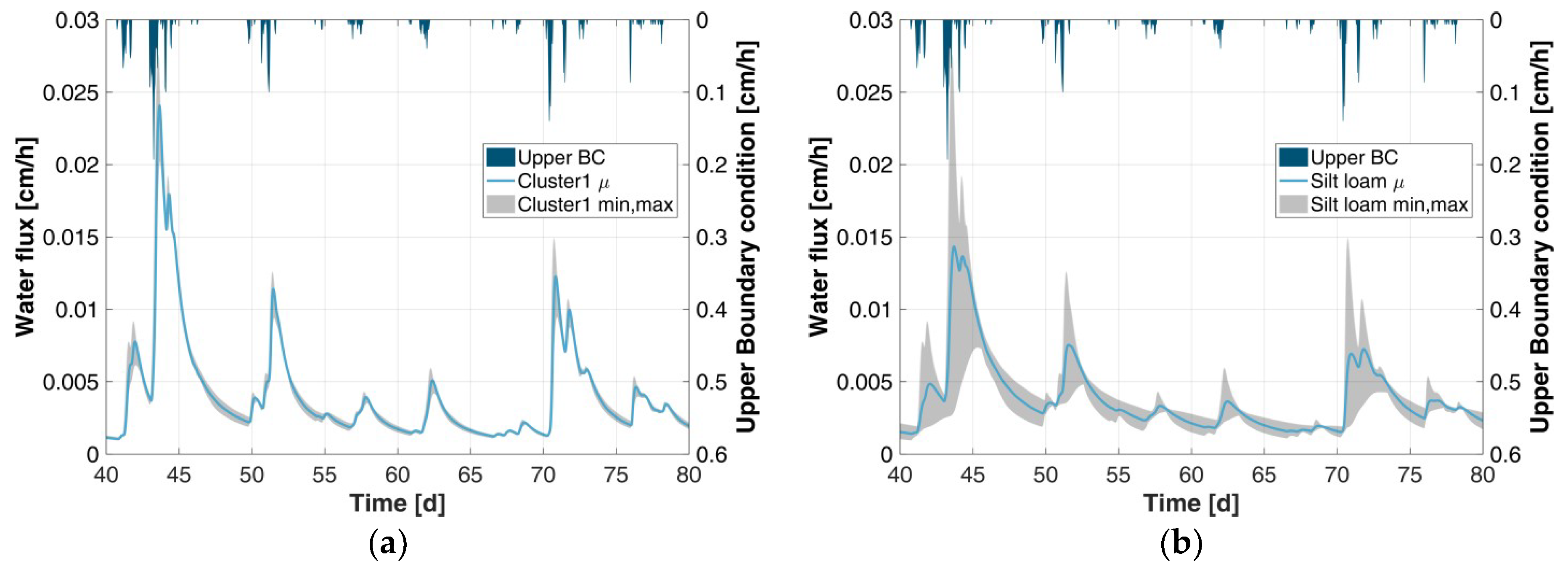
Figure 4 shows the reference time series of the water flux based on DBC at a depth of 40 cm for cluster 1 (Figure 4a) and the average time series for the corresponding USDA class silt loam (Figure 4b), which is located in the same region of the texture triangle. In addition to these two time series, the minimum and the maximum flux for each time step are shown. These time step based minima and maxima were calculated from all class members of cluster 1, as well as for the USDA class members of “silt loam”. Obviously, the bandwidth of water flux is enormously higher in the USDA classification when compared to the new classification system. Such large bandwidths can lead to high uncertainties or even to implausible results in hydrological model applications. The bandwidth of the new classification system on the other hand is very narrow, which also indicates that the representative time series is a valid description of the class.
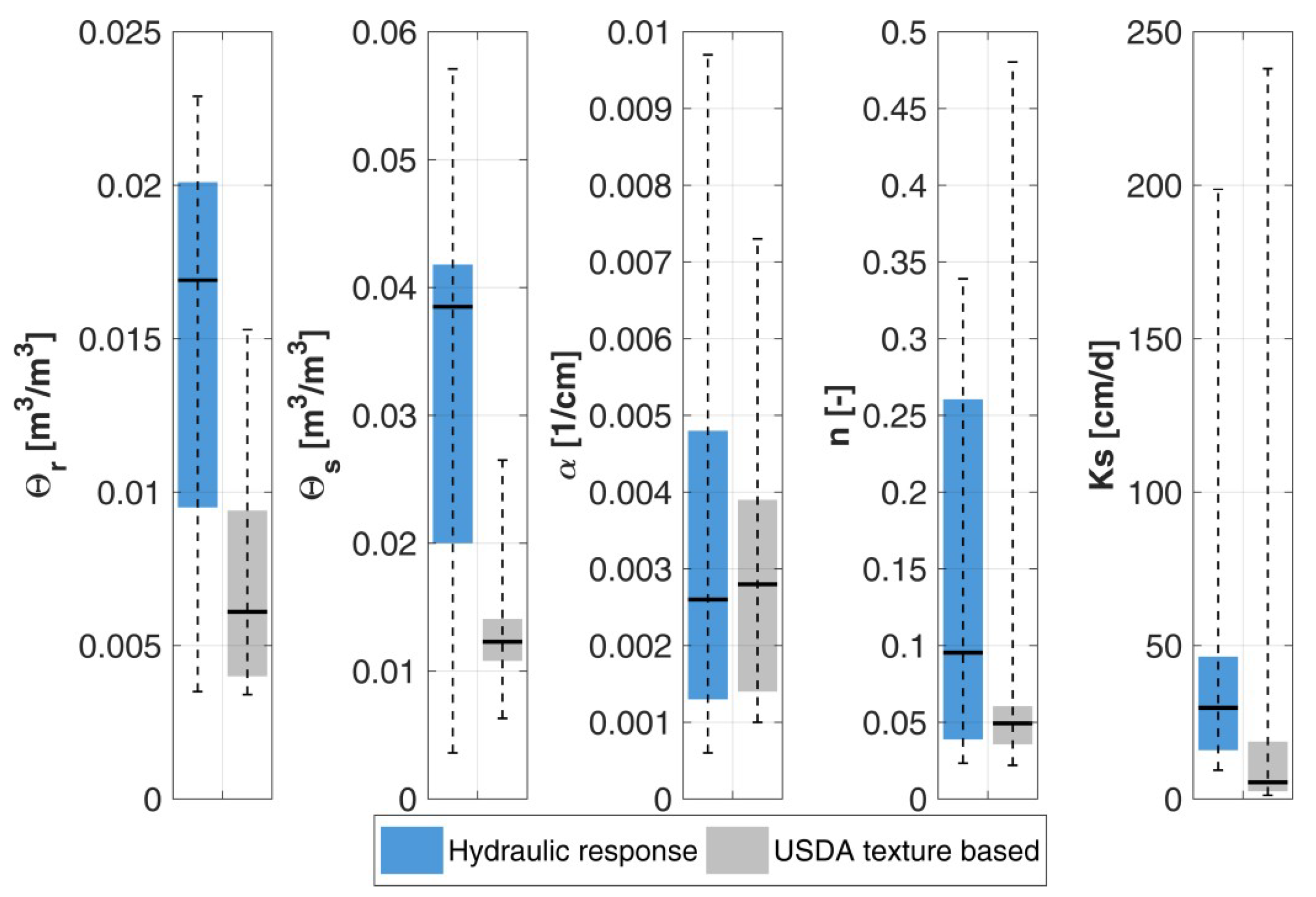
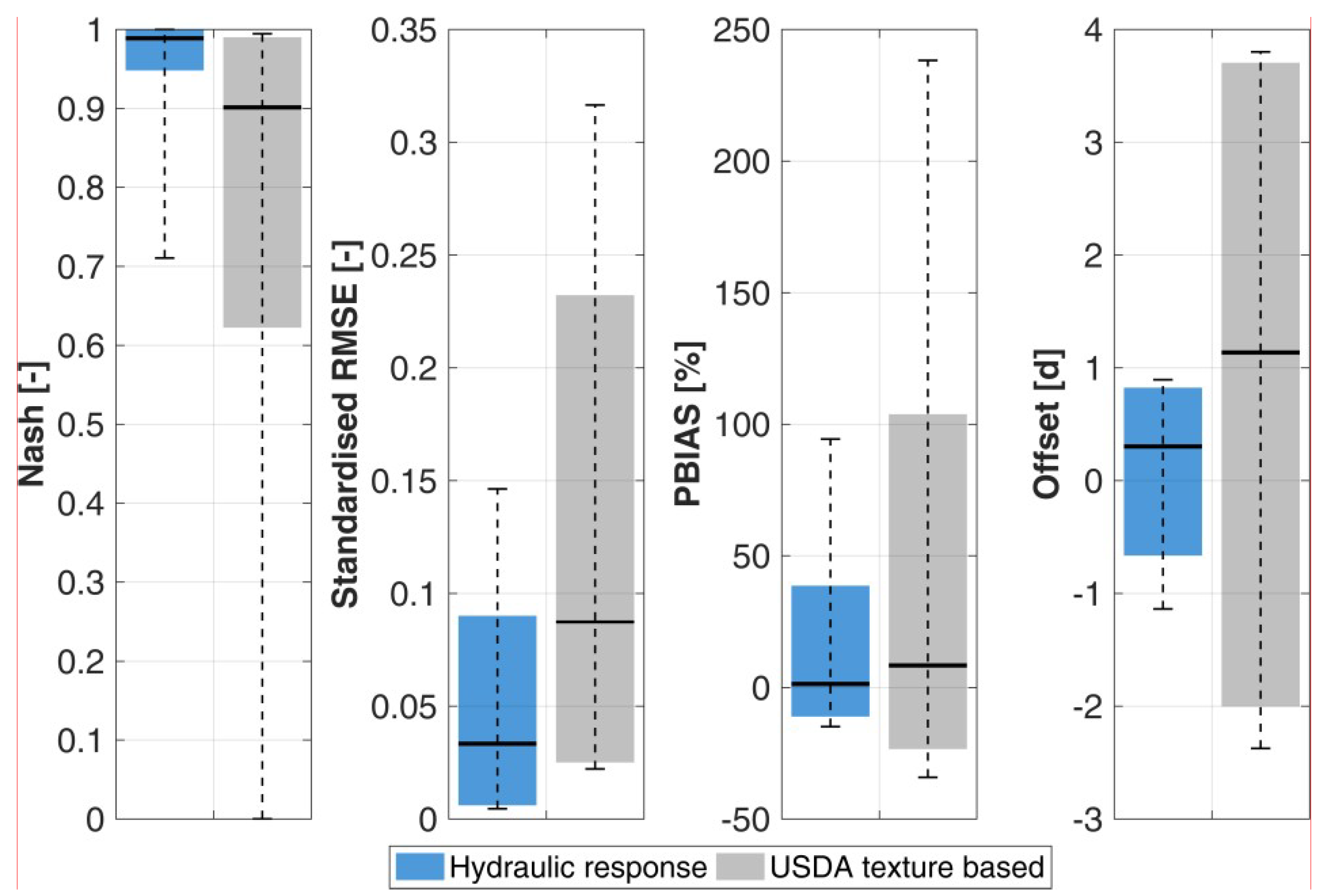
The bandwidth of the VGP and Ks values within the new classes were analysed and compared to the corresponding bandwidth of the parameters within the USDA classes (see Figure 5). Further, the water flux simulations for each class were evaluated regarding homogeneity (see Figure 6). This was done by comparing each time series with the average time series of the class and by calculating different quality criteria for each time series (see Section 2.6). The mean values of each quality criteria were calculated class wise. Figure 6 shows these average values (black horizontal lines), in addition to the bandwidth of the class values. Interestingly, the bandwidth of the VGP and Ks values (Figure 5) are smaller for the USDA classification when compared to the bandwidth of the corresponding parameters for the classification based on hydraulic behaviour. Obviously, the texture based USDA system leads to more similar VGP and Ks-values. In contrast to this, but analogously to Figure 4, all of the quality criteria evaluated for the classification system based on hydraulic behaviour are much better than the criteria based on the USDA system (Figure 6). This leads to the conclusion that: (1) even if the VGP by individual comparison are more different, the simulated water flux can be more similar; and, (2) parameterisation based on hydraulic behaviour should be preferred for hydrological model applications.
4. Discussion
In this study, a new soil classification system was presented as tailored for hydrological modelling. Due to the data scale, the soil hydraulic parameterisation of such models is mostly based on the texture based classification, like the USDA system [8]. We showed that simulated time series of water flux for the same USDA class have very large variations. Hence, it is difficult to select representative soil hydraulic parameters that are valid for one entire texture class. The proposed new classification system is motivated in soil hydraulic behaviour. More than one-million simulated time series of soil water flux in high temporal resolution based on different parameterisation were utilised as inputs for similarity analyses (k-means clustering). The resulting 15 classes showed a different pattern when compared to the USDA texture based classes when visualising the class members in the texture triangle.
It is noteworthy, that our pattern resembles findings of [35], although their research approach was different. They analysed relationships between the saturated hydraulic conductivity and the particle size distribution, which was classified by means of various thresholds. The particle class “sand” was additionally subdivided into five subclasses (“very coarse sand” to “very fine sand”), while the classes “silt” and “clay” remained unchanged. Out of these seven classes, three classes were merged each. This generated 15 different triplets. The information entropy [36], which is a measure of heterogeneity, was calculated for the entire texture triangle for each triplet. The Information Entropy for the triplet that subdivided the texture into the classes “very coarse sand”, “coarse sand”, and “all other” (cf. Figure 2 in [35]) shows a high similarity to the pattern of the soil classification based on hydraulic response found in the study at hand. Possibly, the distinction by heterogeneity with individual consideration of the coarsest sand-classes is a good indicator of soil hydraulic behaviour. The pattern that is classified by [10], on the other hand, differs from the found pattern of the study at hand. From our point of view, the melt down of complex simulations to the mean yearly values of water balance components is avoidable and a too high loss of information when compared to series with a high temporal resolution.
The results of the study at hand were expected to be different to the results of [13], because there are many possible ways to simulate/observe one and the same amount of change in water storage. Two soils with different hydraulic behaviour could possibly come to the same total change in water storage—but on different pathways. This is also significantly dependent on the time period of simulation. For these reasons, we considered the complete time series of water flux in order to use as much information as possible for the clustering. One of the patterns that was elaborated by [13] has similarity to the results of the study at hand (variant of “infiltration & drainage”). Since this variant perhaps holds the highest content of information and accounts both for behaviour of infiltration and for drainage (as storage difference), it is perhaps the most exhaustive variant.
Our first approach of classification is based on simulations with the constant flux upper boundary condition. However, obviously, the determined flux at the upper boundary generates unsaturated conditions in a way that some “extreme” soils (sand, clay) show a similar vertical flux. For this reason, we implemented the second boundary condition with a dynamic flux. We used real measurements of precipitation to be as realistic as possible. With this boundary, we got a similar classification when compared to the simulations with constant flux, but the effect of pure sand and clay in the same class vanished.
Subsequent to the pattern in the texture triangle, the representative time series of water flux for the new classes were compared to the representative time series for USDA texture classification. Note, water flux was selected, since this is the most important variable for hydrologist. This explains why we investigated the performance of the classification system based on water flux as validation criteria—to show that the classification really worked and improved the uncertainties. Of course, it would be a surprise, if the new classification would fail in doing so. However, we are satisfied that we found remarkably lower uncertainties for the new classification. The bandwidth of plotted time series within one and the same class had orders that were of magnitudes higher for the USDA system as for the new system. Apart from that, quality criteria to evaluate the similarity of the time series within one and the same class were clearly better for the system that was proposed in this study. However, it should be noted that the bandwidth of time series as well as the quality criteria are both based on the soil water flux.
5. Conclusions
The new classification helps to fill the gap between complex parameterisation and the hydrologist daily routine (having only coarse spatial data). Note, our findings are based on simulations within a uniform soil with a zero slope surface and without ponding. Although the new classification system is very promising, we have to keep in mind that one shortcoming is the simplification regarding soil structure and bulk density. For further research, it is highly interesting to also include evapotranspiration and/or different bulk densities into the simulations. Evapotranspiration is dependent on the geographic location, on vegetation type, and on the season. Hence, one has to generate a lot of more variants, also in combination with different bulk densities.
With the new classification, hydrological models can utilize multiple parameter sets with the weighted averages of simulated soil water fluxes instead of questionable effective parameter sets. The authors, to parameterise and apply a novel model prototype of soil water movement based on discrete particles, will use the new classification results. This model prototype is the very first step within the on-going DFG (German Research Foundation) project D-SWAP (Integrating hydrological, hydro-geological, soil-physical and hydrodynamic processes by means of particle based simulations. Project number 380258232).
Author Contributions
Conceptualization, P.K.; methodology, P.K.; software, P.K., M.G. and M.S.; validation, P.K. and M.G.; formal analysis, P.K. and M.G.; investigation, P.K. and M.G.; resources, P.K.; data curation, P.K. and M.G.; writing—original draft preparation, P.K., M.G.; writing—review and editing, M.S. and G.M.; visualization, P.K. and M.G.; supervision, G.M.; project administration, P.K.; funding acquisition, P.K.
Funding
We thank the German Research Foundation (DFG) for funding.
Conflicts of Interest
The authors declare no conflict of interest.
References
- Blöschl, G.; Sivapalan, M. Scale issues in hydrological modelling: A review. Hydrol. Process. 1995, 9, 251–290. [Google Scholar] [CrossRef]
- Hopmans, J.W.; Nielsen, D.R.; Bristow, K.L. How useful are small-scale soil hydraulic property measurements for large-scale vadose zone modeling? In Environmental Mechanics: Water, Mass and Energy Transfer in the Biosphere; AGU: Washington, DC, USA, 2002; ISBN 0-87590-988-4. [Google Scholar]
- Beven, K. Linking parameters across scales: Subgrid parameterizations and scale dependent hydrological models. Hydrol. Process. 1995, 9, 507–525. [Google Scholar] [CrossRef]
- Bronstert, A.; Bárdossy, A. The role of spatial variability of soil moisture for modelling surface runoff generation at the small catchment scale. Hydrol. Earth Syst. Sci. 1999, 3, 505–516. [Google Scholar] [CrossRef]
- Hasenauer, S.; Komma, J.; Parajka, J.; Wagner, W.; Blöschl, G. Bodenfeuchtedaten aus Fernerkundung für hydrologische Anwendungen. Österr Wasser- und Abfallw 2009, 61, 117–123. [Google Scholar] [CrossRef] [Green Version]
- Kreye, P. Mesoskalige Bodenwasserhaushaltsmodellierung mit Nutzung von Grundwassermessungen und Satellitenbasierten Bodenfeuchtedaten. Ph.D. Dissertation, Technische Universität Braunschweig, Braunschweig, Germany, 2015. [Google Scholar]
- Kreye, P.; Meon, G. Subgrid spatial variability of soil hydraulic functions for hydrological modelling. Hydrol. Earth Syst. Sci. 2016, 20, 2557–2571. [Google Scholar] [CrossRef] [Green Version]
- Davis, R.O.E.; Bennett, H.H. Grouping of Soils on the Basis of Mechanical Analysis; U.S. Department of Agriculture: Washington, DC, USA, 1927.
- Twarakavi, N.K.C.; Šimůnek, J.; Schaap, M.G. Can texture-based classification optimally classify soils with respect to soil hydraulics? Water Resour. Res. 2010, 46, W01501. [Google Scholar] [CrossRef]
- Bormann, H. Towards a hydrologically motivated soil texture classification. Geoderma 2010, 157, 142–153. [Google Scholar] [CrossRef]
- Diekkrüger, B.; Arning, M. Simulation of water fluxes using different methods for estimating soil parameters. Ecol. Model. 1995, 81, 83–95. [Google Scholar] [CrossRef]
- Brooks, R.H.; Corey, A.T. Hydraulic Properties of Porous Media; Colorado State University: Fort Collins, CO, USA, 1964. [Google Scholar]
- Groenendyk, D.G.; Ferré, T.P.A.; Thorp, K.R.; Rice, A.K. Hydrologic-Process-Based Soil Texture Classifications for Improved Visualization of Landscape Function. PLoS ONE 2015, 10, e0131299. [Google Scholar] [CrossRef] [PubMed]
- Šimůnek, J.; van Genuchten, M.T.; Šejna, M. HYDRUS 1D Software Package for Simulating the One-Dimensional Movement of Water, Heat, and Multiple Solutes in Variably-Saturated Media. IGWMC-TPS70 Version 4.08; Colorado School of Mines: Golden, CO, USA, 2009. [Google Scholar]
- Van Genuchten, M.T. A Closed-form Equation for Predicting the Hydraulic Conductivity of Unsaturated Soils. Soil Sci. Soc. Am. J. 1980, 44, 892–898. [Google Scholar] [CrossRef]
- Richards, L.A. Capillary conduction of liquids through porous mediums. Physics 1931, 1, 318–333. [Google Scholar] [CrossRef]
- Lloyd, S. Least squares quantization in PCM. IEEE Trans. Inf. Theory 1982, 28, 129–137. [Google Scholar] [CrossRef] [Green Version]
- Arthur, D.; Vassilvitskii, S. K-means++: The advantages of careful seeding. In Proceedings of the 18th Annual ACM-SIAM Symposium on Discrete Algorithms, New Orleans, LA, USA, 7–9 January 2007. [Google Scholar]
- Schaap, M.G.; van Leij, J.F.; van Genuchten, M.T. ROSETTA: A computer program for estimating soil hydraulic parameters with hierarchical pedotransfer functions. J. Hydrol. 2001, 2001, 163–176. [Google Scholar] [CrossRef]
- Leij, F.; William, J.; van Genuchten, M.; Williams, J. The UNSODA Unsaturated Soil Hydraulic Database: User’s Manual; National Risk Management Research Laboratory, Office of Research and Development, U.S. Environmental Protection Agency: Cincinnati, OH, USA, 1996.
- Nemes, A.; Schaap, M.; Leij, F.; Wösten, J. Description of the unsaturated soil hydraulic database UNSODA version 2.0. J. Hydrol. 2001, 251, 151–162. [Google Scholar] [CrossRef]
- Jury, W.A.; Horton, R. Soil physics, 6th ed.; J. Wiley: Hoboken, NJ, USA, 2004; ISBN 9780471059653. [Google Scholar]
- Wösten, J.H.M.; van Genuchten, M.T. Using Texture and Other Soil Properties to Predict the Unsaturated Soil Hydraulic Functions. Soil Sci. Soc. Am. J. 1988, 52, 1762–1770. [Google Scholar] [CrossRef]
- Van Genuchten, M.T.; Nielsen, D.R. On Describing and Predicting the Hydraulic Properties of Unsaturated Soils. Ann. Geophys. 1985, 615–628. [Google Scholar]
- Mualem, Y. A new model for predicting the hydraulic conductivity of unsaturated porous media. Water Resour. Res. 1976, 12, 513–522. [Google Scholar] [CrossRef]
- Børgesen, C.D.; Iversen, B.V.; Jacobsen, O.H.; Schaap, M.G. Pedotransfer functions estimating soil hydraulic properties using different soil parameters. Hydrol. Process. 2008, 22, 1630–1639. [Google Scholar] [CrossRef]
- Pérez-Cutillas, P.; Barberá, G.G.; Conesa-García, C. Effects of the texture and organic matter values in the estimation of the soil water content at a regional scale. Cuadernos de Investigación Geográfica CIG 2018, 44, 697–718. [Google Scholar] [CrossRef]
- Schaap, M.G.; Leij, F.J.; van Genuchten, M.T. Neural Network Analysis for Hierarchical Prediction of Soil Hydraulic Properties. Soil Sci. Soc. Am. J. 1998, 62, 847–855. [Google Scholar] [CrossRef]
- Skeel, R.D.; Berzins, M. A Method for the Spatial Discretization of Parabolic Equations in One Space Variable. SIAM J. Sci. Stat. Comput. 1990, 11, 1–32. [Google Scholar] [CrossRef]
- Sturges, H.A. The Choice of a Class Interval. J. Am. Stat. Assoc. 1926, 21, 65–66. [Google Scholar] [CrossRef]
- Pearson, K. Note on Regression and Inheritance in the Case of Two Parents. Proc. R. Soc. Lond. 1895, 58, 240–242. [Google Scholar] [CrossRef]
- Nash, J.E.; Sutcliffe, J.V. River Flow Forecasting through Conceptual Models. J. Hydrol. 1970, 10, 282–290. [Google Scholar]
- Legates, D.R.; McCabe, G.J. Evaluating the use of “goodness-of-fit” Measures in hydrologic and hydroclimatic model validation. Water Resour. Res. 1999, 35, 233–241. [Google Scholar] [CrossRef] [Green Version]
- Hall, M.J. How well does your model fit the data? J. Hydroinform. 2001, 3, 49–55. [Google Scholar] [CrossRef] [Green Version]
- García-Gutiérrez, C.; Pachepsky, Y.; Martín, M.Á. Saturated Hydraulic Conductivity and Textural Heterogeneity of Soils. Hydrol. Earth Syst. Sci. Discuss. 2018, 22, 3923–3932. [Google Scholar] [CrossRef]
- Shannon, C.E. The Mathematical Theory of Communication; University of Illinois Press: Baltimore, MD, USA, 1948; ISBN 9780252725463. [Google Scholar]
Figure 1.
General procedure of soil classification by means of their hydraulic behaviour.

Figure 2.
Number of Clusters in relation to standardized objective functions. All criteria were set to the same range (0 = no agreement, 1 = perfect agreement). (a) Impulse boundary condition; (b) Dynamic boundary condition. Correlation = Pearson correlation coefficient, RMSE = root mean square error, Nash = model efficiency [32], Agreement = Index of agreement, Mean OF = arithmetic mean out of all objective functions. “Std” denotes for standard deviation.

Figure 3.
(a,b): Texture triangle with classification results for 15 classes (coloured patterns) based on hydraulic response in comparison to the established United States Department of Agriculture (USDA) classification [8]. (a): Impulse boundary condition (IBC); (b): Dynamic boundary condition (DBC). (c,d): Representative time series of water flux for the 15 classes based on IBC (c) and DBC (d). The legend numbering is in consistence with Table 1.


Figure 4.
(a) Representative time series of cluster 1 of the classification based on hydraulic behaviour (blue line) for the dynamic boundary condition. Further, the minima and maxima out of all class members are shown for each time step (grey area). (b) The same analyse for the class members of “silt loam” of the USDA classification.

Figure 5.
Standard deviation of van Genuchten Parameters and Ks values within the classes (blue = evaluation based on hydraulic response classes; grey = based on USDA classes). The horizontal black lines show the median. The boxes show the 25% and 75% percentiles and the whiskers symbolise the minima and maxima.

Figure 6.
Bandwidth of the quality criteria Nash, RMSE (standardized), PBIAS (percentage error) and Offset (blue = evaluation based on hydraulic response classes; grey = based on USDA classes). The optimal value of Nash is one; the optimal values of RMSE, PBIAS, and Offset are zero. The horizontal black lines show the mean quality values of all classes. The boxes show the mean values ± two times standard deviation (cut at a value of one) and the whiskers symbolise the minimum and maximum values.


Table 1.
Representative van Genuchten parameters of the 15 classes of the classification based on hydraulic response with dynamic boundary condition.
Table 1.
Representative van Genuchten parameters of the 15 classes of the classification based on hydraulic response with dynamic boundary condition.
| Nr | Θr (m³∙m−3) | Θs (m³∙m−3) | α (m−1) | n (-) | Ks (m∙s−1) |
|---|---|---|---|---|---|
| 1 | 0.049 | 0.448 | 0.005 | 1.721 | 5.09 × 10⁻⁶ |
| 2 | 0.051 | 0.479 | 0.006 | 1.694 | 4.98 × 10⁻⁶ |
| 3 | 0.065 | 0.463 | 0.006 | 1.660 | 2.55 × 10⁻⁶ |
| 4 | 0.069 | 0.468 | 0.006 | 1.636 | 2.08 × 10⁻⁶ |
| 5 | 0.075 | 0.469 | 0.007 | 1.612 | 1.50 × 10⁻⁶ |
| 6 | 0.087 | 0.471 | 0.008 | 1.539 | 1.27 × 10⁻⁶ |
| 7 | 0.093 | 0.479 | 0.010 | 1.453 | 1.50 × 10⁻⁶ |
| 8 | 0.101 | 0.499 | 0.015 | 1.300 | 2.43 × 10⁻⁶ |
| 9 | 0.103 | 0.505 | 0.020 | 1.158 | 1.97 × 10⁻⁶ |
| 10 | 0.108 | 0.511 | 0.018 | 1.153 | 2.08 × 10⁻⁶ |
| 11 | 0.074 | 0.399 | 0.024 | 1.300 | 1.04 × 10⁻⁶ |
| 12 | 0.073 | 0.384 | 0.027 | 1.263 | 1.50 × 10⁻⁶ |
| 13 | 0.071 | 0.372 | 0.025 | 1.276 | 1.62 × 10⁻⁶ |
| 14 | 0.053 | 0.376 | 0.032 | 2.582 | 4.12 × 10⁻⁵ |
| 15 | 0.056 | 0.373 | 0.031 | 3.347 | 8.61 × 10⁻⁵ |
© 2019 by the authors. Licensee MDPI, Basel, Switzerland. This article is an open access article distributed under the terms and conditions of the Creative Commons Attribution (CC BY) license (http://creativecommons.org/licenses/by/4.0/).
Share and Cite
MDPI and ACS Style
Kreye, P.; Gelleszun, M.; Somasundaram, M.; Meon, G. Classification of Hydrological Relevant Parameters by Soil Hydraulic Behaviour. Geosciences 2019, 9, 206. https://doi.org/10.3390/geosciences9050206
AMA Style
Kreye P, Gelleszun M, Somasundaram M, Meon G. Classification of Hydrological Relevant Parameters by Soil Hydraulic Behaviour. Geosciences. 2019; 9(5):206. https://doi.org/10.3390/geosciences9050206
Chicago/Turabian StyleKreye, Phillip, Marlene Gelleszun, Manickam Somasundaram, and Günter Meon. 2019. "Classification of Hydrological Relevant Parameters by Soil Hydraulic Behaviour" Geosciences 9, no. 5: 206. https://doi.org/10.3390/geosciences9050206
Note that from the first issue of 2016, this journal uses article numbers instead of page numbers. See further details here.