Recognize the Little Ones: UAS-Based In-Situ Fluorescent Tracer Detection


Institute of Landscape Ecology, University of Münster, Heisenbergstr. 2, 48149 Münster, Germany
*
Author to whom correspondence should be addressed.
Drones 2019, 3(1), 20; https://doi.org/10.3390/drones3010020
Submission received: 21 December 2018
/
Revised: 16 February 2019
/
Accepted: 17 February 2019
/
Published: 20 February 2019
Abstract
:In ecological research, a key interest is to explore movement patterns of individual organisms across different spatial scales as one driver of biotic interactions. While various methods exist to detect and record the presence and movements of individuals in combination with UAS, addressing these for smaller animals, such as insects, is challenging and often fails to reveal information on potential interactions. Here, we address this gap by combining the UAS-based detection of small tracers of fluorescent dyes by means of a simple experiment under field conditions for the first time. We (1) excited fluorescent tracers utilizing an UV radiation source and recorded images with an UAS, (2) conducted a semi-automated selection of training and test samples to (3) train a simple SVM classifier, allowing (4) the classification of the recorded images and (5) the automated identification of individual traces. The tracer detection success significantly decreased with increasing altitude, increasing distance from the UV radiation signal center, and decreasing size of the fluorescent traces, including significant interactions amongst these factors. As a first proof-of-principle, our approach has the potential to be broadly applicable in ecological research, particularly in insect monitoring.

1. Introduction
A fundamental question driving ecological research is finding explanations that lead to species interactions and their spatial distributions, from global down to local scale [1].
Today, various methods of remote sensing (such as radio-telemetry, harmonic radar or LIDAR) are used for detecting and recording the movements of organisms in their natural environments [2,3,4,5,6]. However, these methods often require the attachment of devices on every single individual every single individual, and are time and/or cost consuming, especially for investigations of larger insect populations. Alternatively, the use of fluorescent powder dyes was successfully applied as a non-invasive method for vertebrates [7,8,9,10] and invertebrates [11,12,13]. It proved to be an affordable method while allowing the detection of many individuals in parallel [12]. In principle, the fluorescent tracer dye emits signals when illuminated by a UV-light source, which can be detected optically or perceived visually. Thus, the method allows the detection of animal interactions (e.g., flower visits of pollinators [13,14,15]) or tracking movements indirectly, e.g., by following tracks until full signal decay [7,16,17,18,19]. However, manually searching for fluorescent powder in the field, such as residues on flowers using UV radiation flashlights, is very labor-intensive and time-consuming.
Automated image processing and object-based analysis techniques are by now well-established in the remote sensing community. Moreover, recent technical trends, including minimization of high-quality sensors, have led to new possibilities in the use of unmanned aerial systems (UAS) in various fields and applications [20]. In particular, UAS are now used in ecology and agriculture in a spectrum of research topics [20,21], such as plant identification [22] and weed management [23,24], or pest control and insect monitoring [25,26,27,28,29].
With the advantage of being able to fly at low altitudes, very high-resolution data can be generated flexibly in time and space and thus according to the requirements of the user [20,30]. Therefore, remote sensing based on using UAS can provide new capabilities to capture fluorescent traces on plants over larger spatial scales. Recent studies already used UAS to detect locusts combined with strobe-based optical methods [31,32]. However, to our knowledge neither any study tested the detection of fluorescent powder dye by UAS derived image data so far, nor used an automated classification and object identification approach to provide tracking information on insect movement from such detections.
Here we aimed to combine these methods and scrutinized if such a detection, automated identification and classification of fluorescent tracer dyes by UAS and post-processing is principally possible and feasible. To answer these questions, we developed a standardized experimental protocol under simple, low-altitude field-conditions as a first proof-of-principles. We tested three parameters in our set-up, which we determined to be highly influential on the efficiency of fluorescent tracer detection: (a) the distance between the UAS camera sensor and a fluorescent tracer, (b) the distance between the projection center on the ground of a UV radiation source spotlight and the fluorescent tracer (i.e., this measure determines the excitation intensity of the fluorescent tracer) and (c) the size of the fluorescent tracer.
We hypothesize that:
- detection probability decreases with increasing distance between the UAS camera sensor and the fluorescent tracer (DTS),
- detection probability decreases with increasing distance between the projection center on the ground of a UV radiation source spotlight and the fluorescent tracer (DTL),
- detection probability increases with increasing size of the fluorescent tracer.
2. Materials and Methods
2.1. Experimental Design & Data Collection
Four patterns were created with a custom R script using package raster [33], R-version 3.1.3 [34], creating a raster with 200 columns and 200 rows yielding a quadratic cell size of one mm² (Supplementary Materials-Appendix A). Hereof, 1% of the (i.e., 400) cells were randomly selected to receive a fluorescent tracer marking. We aimed to use three different tracer dyes, yielding 133 cells per dye. From the selected raster cells a subset of cells per dye (20%, i.e., 26 cells) was extended by selecting the neighboring cells above, to the right, and above right of these cells yielding a second cell size of four mm² (Table 1). The raster was printed on DIN A2 paper sheets sustaining cell edge lengths of one [mm]. The selected cells were filled with a paste of an ethanol water mixture (70% vol. ethanol) and the fluorescent dyes (GloMania, UVPP-SET-10, dyes yellow, green and neon pink) resulting in fluorescent traces when dried. These paper sheets were glued on cardboards to ensure a standardized smooth surface.
All four cardboards were placed outdoors on mowed lawn surface in the shape of an imaginary rectangle, leaving 10 cm between the borders of each sheet. The UV-light source (custom made, Supplementary Materials-Appendix B) was held by hand and its focus aligned with the center of the object level. The light source distance (i.e., height) to the sheets was approximately 1.5 m. Data collection took place at night, by hovering over the sheets with a quadcopter-type UAS (platform: DJI Mavic Pro, DJI Innovations, Shenzhen, China) holding a Red-Green-Blue-camera (RGB-camera; DJI FC220. DJI Enterprise 2017), see Figure 1, with a focal length of 5 mm and a 1/2.3”-CMOS (DJI Enterprise 2017). The exposure was set to 1/200 s to gather fluorescence signals without much shaking due to the camera gimbal movement. Photosensitivity and aperture were controlled by the cameras internal software and set to ISO-1600; f = 2.2.
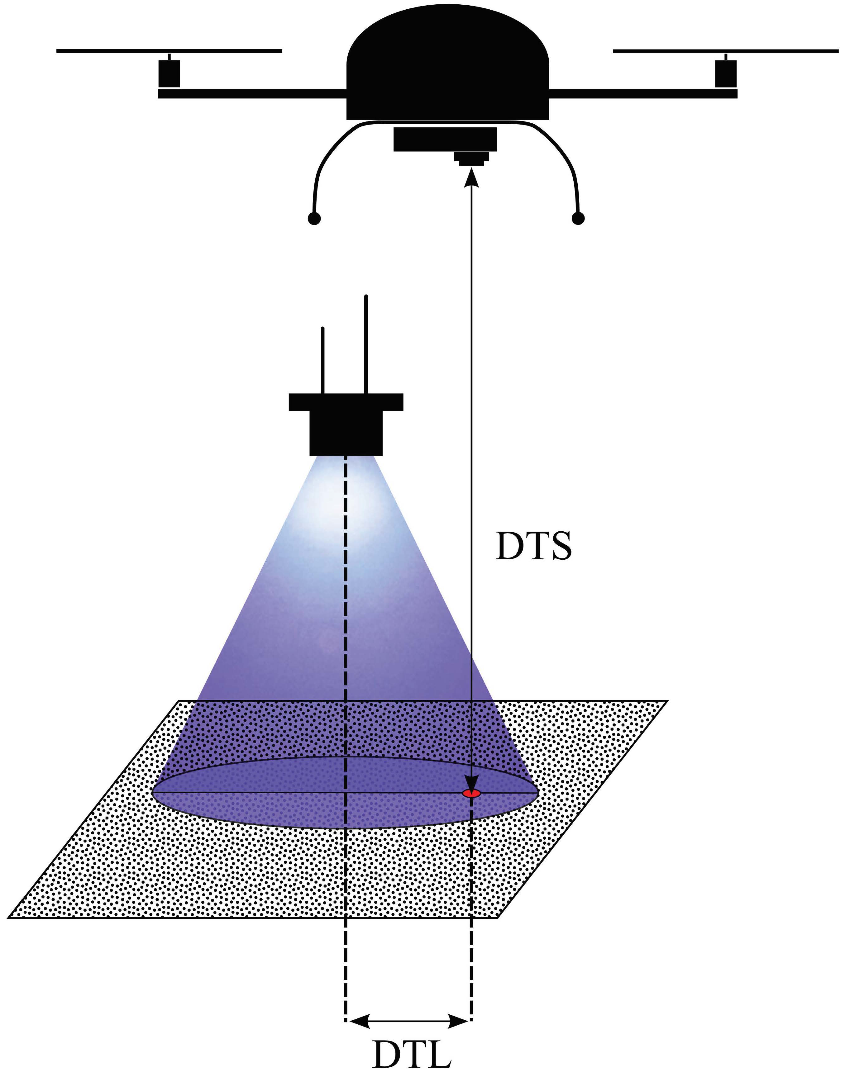
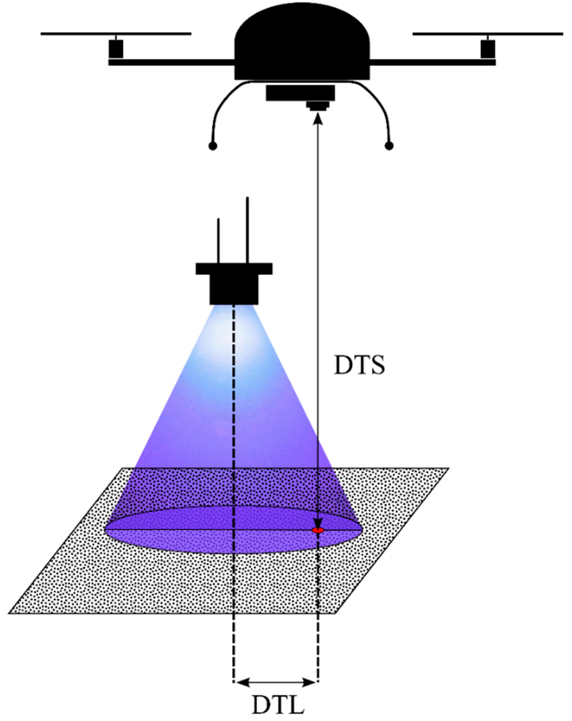
To analyze the maximum spatial resolution of the set-up, we considered two different heights from which image shots were taken, those were measured as the distance from the object to the camera sensor (DTS; Figure 1). More specifically, we took images at 2.2–2.7 m (distance class 1) and 3.0–3.65 m (distance class 2), corresponding to a spatial resolution of 0.67–0.83 mm and 0.94–1.13 mm, respectively. In addition, we calculated the distance from the center of the light source to each individual tracer (see details below; DTL; Figure 1).
During data selection, we accepted only images with visible fluorescence. The traces were sufficiently illuminated and no loss of quality due to focus or camera shake was discernible. This resulted in two images of distance class 1 and eight images of distance class 2 (Table 1). In addition, the subsequent image data processing concentrated on the yellow dye (i.e., fluorescein), omitting the green and neon pink dye because of insufficient fluorescence signals from the latter two (Supplementary Materials-Appendix B). No additional image pre-processing was applied.
2.2. Image Data Processing
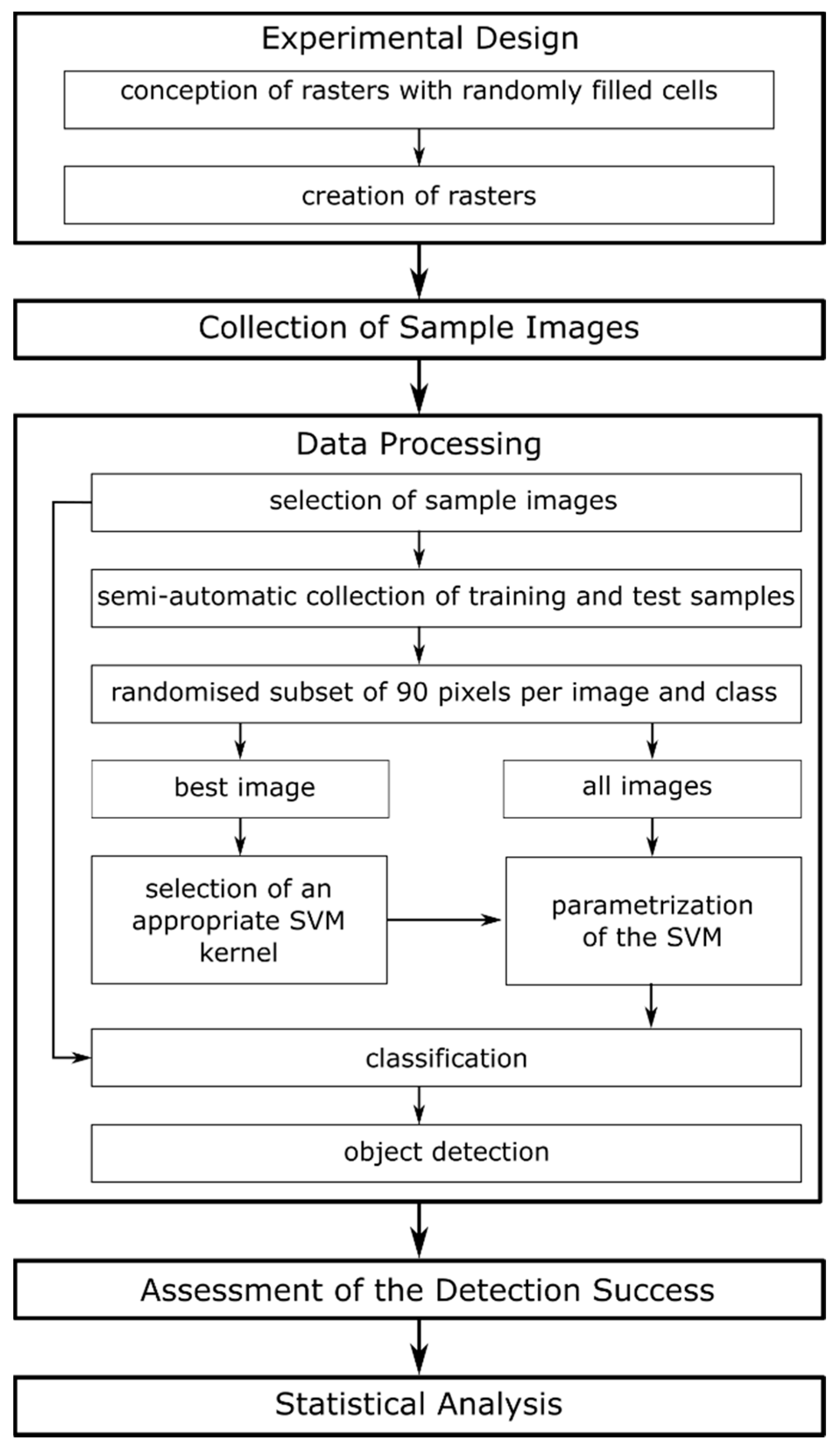
Data analysis encompassed the selection of training and a test sample dataset of a fluorescent trace, classification of the fluorescent trace pixels in comparison to background pixels, and object detection (Figure 2):
Training and test sample pixels were selected manually: Regarding the fluorescent traces, a threshold-based approach considering the three image bands of the RGB images was applied. A pixel representing a fluorescent trace was selected and all pixels diverging maximal five values in each band, starting from the selected pixel, were added to the selection automatically. This approach was stopped when the manual selection of a pixel representing a fluorescent trace would have led to the automatic selection of pixels representing background. Background pixels were sampled stratified to guarantee that both spectrally distinct features (the paper and other backgrounds) were equally represented by the sample. Pixels representing paper were selected using circular regions with a diameter of 20 pixels, manually placed on the image regions representing paper along a raster with a cell size of 20 pixels. These circular regions were chosen such that the sample represents the illumination gradient while emphasizing the regions where the paper was illuminated. These light regions were spectrally similar to the fluorescent traces and therefore, pixels in this spectral subspace are most important for the construction of the support vectors (see below). Other background pixels were sampled using two one-pixel-wide lines placed horizontally across the image and two additional one-pixel-wide lines recording the region at the paper margin. From the generated samples, we randomly selected pixels according to the “30p rule” [35] resulting in a total sample size of 90 pixels representing the fluorescent traces and 45 pixels representing paper and other backgrounds, respectively. Samples were derived from each image according to this procedure using GIMP 2.8.18 [36]. Random subsets from these were sampled using R. We provide R scripts for image classification and object detection in a self-written R-package [34] “TraceIdentification” (v. 0.0.0.9000; available online at GitHub: https://github.com/henningte/TraceIdentification) (Supplementary Materials-Appendix A). Further R-packages used to conduct the data processing were EBImage [37], sinkr [38], Hmisc [39], doParallel [40], foreach [41], caret [42].
Image classification was conducted using support vector machines (SVM) as classifiers. SVM is known to perform well with small sample sizes [35] and enable the construction of nonlinear decision boundaries. Furthermore, Reference [43] successfully used SVM for classification purposes using images from fluorescence microscopy. Since the envisaged scope of our method is assumed to result in similar image data and represents a similar detection task (small features), it is reasonable to assume that SVMs are suitable classifiers in this case. A two-stage approach was used to select the optimal kernel and fit the parameters of the SVM for the classification task. First, using the training and test sample derived from the best quality image (maximum fluorescence and image scale, least noise), the SVM was constructed in four approaches, each using a different kernel function (linear, radial and homogenous sigmoid). The parameters of each SVM were fitted by a grid search approach [44], using R package e1071, function best.svm, V 1.6-7 [45], whereby the cost parameter (C) was varied in a first step in the interval 2−10; 2−8; …; 210 and in a finer step in the interval C1 - 1.2; C1 - 1.0; …; C1; …; C1 + 1.0; C1 + 1.2, with C1 being the cost parameter of the first approach and all assessed values for the cost parameter > 0. The parameters of the kernel functions were fitted - if necessary - in the intervals: γ ∈ [2−20; 2−18; … ; 26] [44]. The kernel resulting in the best accuracy for the fluorescence tracer in a 10-fold cross validation approach was selected (Supplementary Materials-Appendix A). If more than one kernel resulted in the best accuracy, the simplest kernel was selected. In the second stage, an SVM for each sample image was fitted using the selected kernel and the above-described grid search approach. We calculated the total classification accuracy and the classification accuracy relating to each class (i.e., fluorescent tracer and background) as measures for classification performance (Supplementary Materials-Appendix A).
2.3. Detection Success and Statistics
In a first step, the quality control of the trace detection process, i.e. the successful classification of the fluorescent traces by the chosen SVM, was performed manually by comparing the classified images with the corresponding raster template originals using QGIS [46]. It was only tested if a fluorescent trace was successfully classified (at least one of the corresponding pixels). From each image the successful identified and non-identified tracers were counted. To achieve this, the classified images and the raster templates were referenced relative to each other. A point was created for each trace and additionally for the UV radiation source spot projection centers on each of the original images. In the next step, distances could be derived for each trace and the corresponding UV radiation source spot projection center by computing a distance matrix (Supplementary Materials-Appendix A).
For statistical analysis (Supplementary Materials-Appendices C,D), we fitted generalized linear mixed effects models (GLMM) with binomial distribution family, function lmer from package lme4 [47], in order to assess the dependency of the fluorescent trace detection success (binary response) on the following three predictors: The distance between UAS sensor and fluorescent traces (DTS; 2 levels), the UV radiation intensity measured as distance between the UV radiation source spot projection center on the ground and the fluorescent traces (DTL; continuous), the size of the fluorescent traces (size; 2 levels) and interactions between these parameters. The random structure of the models contained image-id depending on DTS, thus accounting for pseudo-replication because individual tracers were not independent from each other. Previous data inspection was done with package MASS [48] and fitdistrplus [49]. Model selection was done by multi-model inference based on Akaike Information Criterion corrected for small sample sizes (AICc) and Akaike weights using the dredge function from package MuMIn [50]. Model validation was performed graphically and by comparing the best model to generalized linear models without random effects structure by AICc. Subsequent to model selection, the significance of predictors was tested by a Wald chi-square test with type II sums of squares using ANOVA function from package car [51]. Data plotting and visualization were done with package effects [52].
3. Results
The kernel function that led to the best classification accuracy was a radial kernel. For all images, the parameters vary between 0.0625 and 1.05 (C) and 0.0625 and 4 (γ). The classifier achieved overall classification accuracies of 99.67% ± 0.54% (n = 10). The mean detection rates per image varied between 37.4% and 55%. Figure 3 gives two examples of the recorded images and the resulting classification results for the considered distance classes.
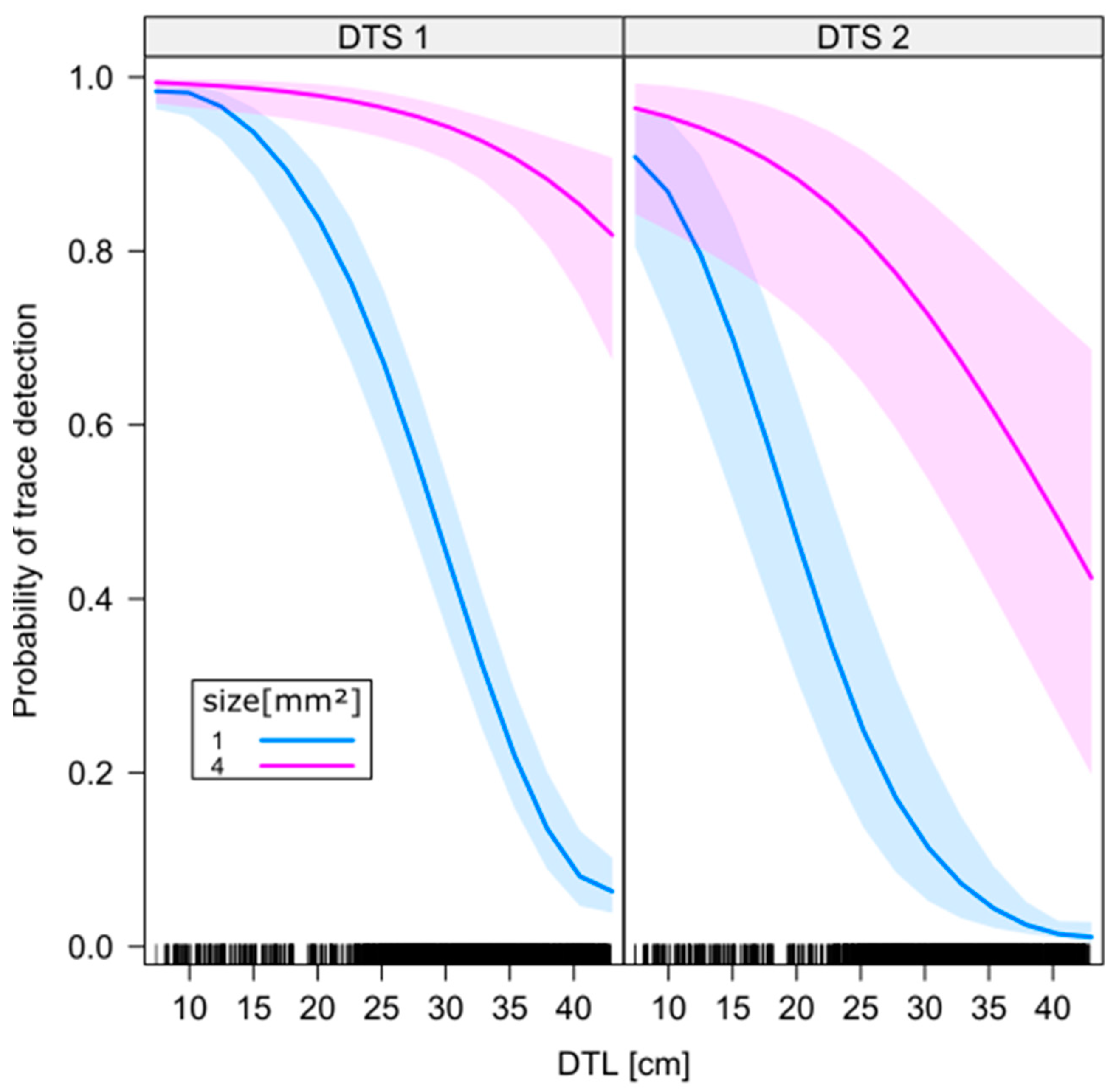
The GLMM with the lowest AICc contains all main parameters and a two-way interaction between the tracer size and the UV radiation intensity (Table 2, Table 3). All main predictors significantly affected detection success (Table 2), but the bigger tracer size alone was not significant (Table 3). In general, small tracer size (red lines in Figure 4) significantly decreased detection success compared to the bigger size (blue lines in Figure 4). In combination with the effect of tracer size, increasing DTL reduced identification success significantly. The interactive effects of tracer size and DTL were attenuated when DTS increased from level one to two, yielding significantly reduced identification success and pointing to the importance of the interplay of all three variables despite the lack of a three-way-interaction term in the best model.
4. Discussion
In general, both, the accuracy of the classification scheme and the results of the statistical analysis, suggest that an automated, UAS-based imaging, subsequent classification, and the identification of fluorescent dyes traces to record movement patterns of organisms (for example pollinators), is technically possible (Table 1, Table 2 and Table 3, Figure 4).
With the featured classification optimization and sampling, the SVM achieved high prediction values for the classification of the used fluorescent dyes leading to almost a complete identification of visually discernible fluorescent traces in the recordings (Table 1). Nevertheless, we account the application of the method to be independent of the program or method used for object classification and identification. Based on the results of the statistical analysis an identification probability of more than 97% can be assumed under optimal conditions, i.e., strong fluorescence signal, traces of a size of around 4 mm2 and a flight height of 2.2 m to 2.7 m (Figure 4).
In sum, all tested main parameters, the distance between the camera sensor and the object level (DTS), the size of the fluorescent trace (size), and the distance between a trace and the center of the UV-light cone at the object level (DTL), significantly affected the identification probability:
Confirming our hypothesis, (i) identification probability decreased with increasing DTS (Figure 4, Table 2). The increased distance (DTS 2; 3 m to 3.65 m) between camera sensor and fluorescent traces led to a significantly lower identification probability of the traces, which presumably occurred due to the lower spatial resolution (0.94–1.13 mm per pixel edge compared to 0.67–0.83 mm per pixel edge at DTS 1) and the lower fluorescent radiation energy that reaches the camera sensor (Table 3, Figure 4).
In this study, the realized flight scenarios, resulting in DTS 1 and DTS 2, were both conducted at very low altitude. In real surveys, when tracers are to be detected in vegetation, we also assume comparably low DTS, relative to altitudes where UAS normally are flown when surveying for pests [53] or breeding birds [54]. However, under these conditions also other methods are applicable, such as camera stands, tripod-based or crane-based options (i.e., a dolly), which may allow for taking images in a more controlled way, without adding the problems derived from UAS-mounted moving cameras. In our approach, we refrained from using such methods, since ecological studies often require more surveyed ground space than a few local spots, which often requires UAS-based surveys [54]. Thus, we tested by directly using an UAS-based approach, to ensure the inclusion of unstable flight conditions. However, we did not test the application in a field survey in a full flight campaign, which needs to be tested in future studies.
In our study, we did not include a higher difficulty of UV trace-detection induced by complex vegetation structure. This might affect the detection success of the UV tracers, whereby more stable conditions during image taking (as derived by the alternative methods) may ensure high detectability and thus may limit the use of a UAS.
Regarding camera settings, we used a large aperture and relatively high film speed (ISO 1600) to allow the use of short exposure times of 1/200 s. This was done to reduce low image qualities due to movements. However, it has to be considered that larger apertures potentially lead to more pronounced optical aberrations of the optical system and therefore may negatively influence image quality, especially at the edges of the images. In contrast, lower apertures in combination with slightly higher exposure times potentially enhance the potential of the presented technique. Therefore, we suggest future investigations consider in depth how image sharpness can be improved by settings of the optical system.
An approach for increasing the DTS, i.e. higher flight levels, while keeping the high spatial resolution constant, is the usage of a professional aerial camera with a larger image sensor size (e.g., medium format). For example, using the PhaseOne iXU 100MP camera sensor would increase the flight height to about 8 m with a comparable GSD of 0.7 mm. However, such professional aerial camera systems are of a heavy weight and thus require more powerful UAS. In this study, the influence of the image sensor size on the classification accuracy was not investigated.
With (ii) increasing DTL, the identification probability decreased significantly (Figure 4, Table 2). This decrease was stronger, the smaller the trace size and the larger the DTS was. This observation can most likely be attributed to the lower intensity of the fluorescence stimulating UV radiation at larger distances to the radiation source. To compensate for this negative effect, we recommend future studies to upregulate light intensity with increasing flight altitude, thus ensuring a constant level of light intensity. Moreover, it is desirable to increase the power of the UV radiation source in general, because higher excitation energies increase the fluorescence of the tracers and therefore the contrast. With this, it could even be possible to compensate for lower resolutions at higher flight heights. Another option could be to also use a light source in addition to the UV radiation source in order to enhance image sharpness. This may support lower film speeds and apertures and therefore could yield a higher signal to noise ratio and fewer aberrations. However, it has to be tested if such a setting would complicate image classification due to lit features that are no fluorescent traces.
We think that all these parameters are worth testing since all suggestions may potentially increase detection success. We suggest analyzing the modulation transfer function (MTF) on test charts using fluorescent tracers as it provides detailed information on image contrast in dependency of both object parameters and parameters of the optical system [55]. By this, it may be possible to offer a procedure on how to choose parameters under different conditions (e.g., size of the traces in different applications or flight height). However, this requires a more detailed and strictly standardized experimental setting.
Our results demonstrate (iii) that identification probability increased with increasing size of the fluorescence tracer (Figure 4, Table 2 and Table 3). The size of the fluorescent traces in relation to the identification probability also interacts significantly with the DTL. This interaction may be caused by a more intense fluorescence and higher detectability of larger traces, even under less intense UV radiation at higher DTS (Figure 4, Table 2 and Table 3). Therefore, it can be assumed that the size of the fluorescent traces is critical for the applicability of the method if the intensity of the UV radiation is low. In this case, differences in the identification success are visible even for small changes in the intensity of the UV radiation. In more realistic flight scenarios, UV-light source and UAS will not be decoupled, but attached to each other, contrary to our approach using a hand-held UV light spot yielding a fixed height to the object level. Thus, when the UV-light spot is attached to a UAS, the DTS and the resulting DTL will be interdependent, both varying with flight altitude. In consequence, we still emphasize to consider interdependency between all three main parameters in future studies.
5. Conclusions
In this study, we provide a first proof-of-principle for the UAS-based detection and identification of small fluorescent dye traits (size range between 1 and 4 mm2) by means of a simple experiment under outdoor light conditions.
Based on the results of the statistical analysis, the highest identification probability in our study is given under optimal conditions of a strong fluorescence signal (low DTL), trace sizes of around 4 mm2 and a low flight height (DTS of 2.2–2.7 m; Figure 4). Since these parameters proved to be interdependent, there is no single parameter to focus on in future studies. We discussed several improvements to be considered, including the promising modulation transfer function (MTF). Since tracer size derived by organisms may vary and cannot be controlled in a standardized way, we also suggest testing more complex set-ups to overcome the limitations of this study.
In summary, we think the proposed method represents the first step to enable automated identification of fluorescent traces and thus facilitate many applications in ecology, such as monitoring of biodiversity, especially of insects, exploring patterns of animal movement, spatial distributions and plant-pollinator interactions.
Supplementary Materials
The following are available online at https://www.mdpi.com/2504-446X/3/1/20/s1. Appendix A: R-code for image classification and object identification, Appendix B: extended Methods, Appendix C: data files, Appendix D: R-code for statistical analysis.
Author Contributions
Conceptualization, J.R.K.L. and D.O.; Data curation, H.T., J.R.K.L., P.G. and F.M.; Formal analysis, H.T. and D.O.; Methodology, H.T., J.R.K.L., P.G., F.M. and D.O.; Software, H.T. and D.O.; Supervision, J.R.K.L. and D.O.; Validation, H.T. and D.O.; Visualization, J.R.K.L.; Writing – original draft, H.T., J.R.K.L. and D.O.
Funding
This research received no external funding. Financial costs were covered from working group funds, raised by the University of Münster, from resources of the government of the German Department North Rhine Westphalia (Nordrhein-Westfalen).
Acknowledgments
We are grateful to the Editor and two anonymous reviewers whose comments helped to improve this manuscript. We thank Ilka Beermann, Markus Frenzel, Joana Gumpert and Charlotte Hurck for assisting in logistics, preparations and fieldwork. Tillmann Buttschardt and Christoph Scherber are acknowledged for valuable feedback. Thorsten Prinz is acknowledged for giving technical support. No third-party funding was involved.
Conflicts of Interest
The authors declare no conflict of interest.
References
- Krebs, C.J. Ecology: Pearson New International Edition: The Experimental Analysis of Distribution and Abundance, 6th ed.; Prentice Hall: Harlow, UK, 2013; ISBN 978-1-292-02627-5. [Google Scholar]
- Woiwod, I.P.; Thomas, C.D.; Reynolds, D.R. Insect Movement: Mechanisms and Consequences, 1st ed.; CABI: Wallingford, UK; New York, NY, USA, 2001; ISBN 978-0-85199-456-7. [Google Scholar]
- Riley, J.R.; Smith, A.D.; Reynolds, D.R.; Edwards, A.S.; Osborne, J.L.; Williams, I.H.; Carreck, N.L.; Poppy, G.M. Tracking bees with harmonic radar. Nature 1996, 379, 29. [Google Scholar] [CrossRef]
- Daniel Kissling, W.; Pattemore, D.E.; Hagen, M. Challenges and prospects in the telemetry of insects. Biol. Rev. Camb. Philos. Soc. 2014, 89, 511–530. [Google Scholar] [CrossRef]
- Hagen, M.; Wikelski, M.; Kissling, W.D. Space Use of Bumblebees (Bombus spp.) Revealed by Radio-Tracking. PLoS ONE 2011, 6, e19997. [Google Scholar] [CrossRef]
- Guan, Z.; Brydegaard, M.; Lundin, P.; Wellenreuther, M.; Runemark, A.; Svensson, E.I.; Svanberg, S. Insect monitoring with fluorescence lidar techniques: Field experiments. Appl. Opt. 2010, 49, 5133–5142. [Google Scholar] [CrossRef]
- Lemen, C.A.; Freeman, P.W. Tracking Mammals with Fluorescent Pigments: A New Technique. J. Mammal. 1985, 66, 134–136. [Google Scholar] [CrossRef] [Green Version]
- Rittenhouse, T.A.G.; Altnether, T.T.; Semlitsch, R.D. Fluorescent Powder Pigments as a Harmless Tracking Method for Ambystomatids and Ranids. Herpetol. Rev. 2006, 37, 188–191. [Google Scholar]
- Orlofske, S.A.; Grayson, K.L.; Hopkins, W.A. The Effects of Fluorescent Tracking Powder on Oxygen Consumption in Salamanders Using Either Cutaneous or Bimodal Respiration. Copeia 2009, 2009, 623–627. [Google Scholar] [CrossRef]
- Furman, B.L.S.; Scheffers, B.R.; Paszkowski, C.A. The use of fluorescent powdered pigments as a tracking technique for snakes. Herpetol. Conserv. Biol. 2011, 6, 473–478. [Google Scholar]
- Foltan, P.; Konvicka, M. A new method for marking slugs by ultraviolet-fluorescent dye. J. Molluscan Stud. 2008, 74, 293–297. [Google Scholar] [CrossRef] [Green Version]
- Rice, K.B.; Fleischer, S.J.; de Moraes, C.M.; Mescher, M.C.; Tooker, J.F.; Gish, M. Handheld lasers allow efficient detection of fluorescent marked organisms in the field. PLoS ONE 2015, 10, e0129175. [Google Scholar] [CrossRef]
- Van Rossum, F.; Stiers, I.; Van Geert, A.; Triest, L.; Hardy, O.J. Fluorescent dye particles as pollen analogues for measuring pollen dispersal in an insect-pollinated forest herb. Oecologia 2011, 165, 663–674. [Google Scholar] [CrossRef]
- Mitchell, R.J.; Irwin, R.E.; Flanagan, R.J.; Karron, J.D. Ecology and evolution of plant–pollinator interactions. Ann. Bot. 2009, 103, 1355–1363. [Google Scholar] [CrossRef] [Green Version]
- Harrison, T.; Winfree, R. Urban drivers of plant-pollinator interactions. Funct. Ecol. 2015, 29, 879–888. [Google Scholar] [CrossRef] [Green Version]
- McDonald, R.W.; St. Clair, C.C. The effects of artificial and natural barriers on the movement of small mammals in Banff National Park, Canada. Oikos 2004, 105, 397–407. [Google Scholar] [CrossRef]
- Townsend, P.A.; Levey, D.J. An Experimental Test of Wether Habitat Corridors Affect Pollen Transfer. Ecology 2005, 86, 466–475. [Google Scholar] [CrossRef]
- Rahmé, J.; Suter, L.; Widmer, A.; Karrenberg, S. Inheritance and reproductive consequences of floral anthocyanin deficiency in Silene dioica (Caryophyllaceae). Am. J. Bot. 2014, 101, 1388–1392. [Google Scholar] [CrossRef] [Green Version]
- Laudenslayer, W.F.; Fargo, R.J. Use of night-vision goggles, light-tags, and fluorescent powder for measuring microhabitat use of nocturnal small mammals. Trans. West. Sect. Wildl. Soc. 1997, 33, 12–17. [Google Scholar]
- Colomina, I.; Molina, P. Unmanned aerial systems for photogrammetry and remote sensing: A review. ISPRS J. Photogramm. Remote Sens. 2014, 92, 79–97. [Google Scholar] [CrossRef] [Green Version]
- Singh, J.S.; Roy, P.S.; Murthy, M.S.R.; Jha, C.S. Application of landscape ecology and remote sensing for assessment, monitoring and conservation of biodiversity. J. Indian Soc. Remote Sens. 2010, 38, 365–385. [Google Scholar] [CrossRef]
- Wang, Z.; Li, H.; Zhu, Y.; Xu, T. Review of Plant Identification Based on Image Processing. Arch. Comput. Methods Eng. 2017, 24, 637–654. [Google Scholar] [CrossRef]
- Rasmussen, J.; Nielsen, J.; Garcia-Ruiz, F.; Christensen, S.; Streibig, J.C. Potential uses of small unmanned aircraft systems (UAS) in weed research. Weed Res. 2013, 53, 242–248. [Google Scholar] [CrossRef]
- López-Granados, F. Weed detection for site-specific weed management: Mapping and real-time approaches. Weed Res. 2011, 51, 1–11. [Google Scholar] [CrossRef]
- Kim, H.G.; Park, J.-S.; Lee, D.-H. Potential of Unmanned Aerial Sampling for Monitoring Insect Populations in Rice Fields. Fla. Entomol. 2018, 101, 330–334. [Google Scholar] [CrossRef]
- Tan, L.T.; Tan, K.H. Alternative air vehicles for sterile insect technique aerial release. J. Appl. Entomol. 2013, 137, 126–141. [Google Scholar] [CrossRef]
- Shields, E.J.; Testa, A.M. Fall migratory flight initiation of the potato leafhopper, Empoasca fabae (Homoptera: Cicadellidae): Observations in the lower atmosphere using remote piloted vehicles. Agric. For. Meteorol. 1999, 97, 317–330. [Google Scholar] [CrossRef]
- Schmale III, D.G.; Dingus, B.R.; Reinholtz, C. Development and application of an autonomous unmanned aerial vehicle for precise aerobiological sampling above agricultural fields. J. Field Robot. 2008, 25, 133–147. [Google Scholar] [CrossRef]
- Park, Y.-L.; Gururajan, S.; Thistle, H.; Chandran, R.; Reardon, R. Aerial release of Rhinoncomimus latipes (Coleoptera: Curculionidae) to control Persicaria perfoliata (Polygonaceae) using an unmanned aerial system. Pest Manag. Sci. 2018, 74, 141–148. [Google Scholar] [CrossRef]
- Zhang, C.; Kovacs, J.M. The application of small unmanned aerial systems for precision agriculture: A review. Precis. Agric. 2012, 13, 693–712. [Google Scholar] [CrossRef]
- Tahir, N.; Brooker, G. Feasibility of UAV Based Optical Tracker for Tracking Australian Plague Locust. In Proceedings of the Australasian Conference on Robotics and Automation, Sydney, Australia, 2–4 December 2009. [Google Scholar]
- Brooker, G.; Randle, J.A.; Attia, M.E.; Xu, Z.; Abuhashim, T.; Kassir, A.; Chung, J.J.; Sukkarieh, S.; Tahir, N. First airborne trial of a UAV based optical locust tracker. In Proceedings of the Australasian Conference on Robotics and Automation, Melbourne, Australia, 7–9 December 2011. [Google Scholar]
- Hijmans, R.J.; van Etten, J.; Cheng, J.; Sumner, M.; Mattiuzzi, M.; Greenberg, J.A.; Lamigueiro, O.P.; Bevan, A.; Bivand, R.; Busetto, L.; et al. Raster: Geographic Data Analysis and Modeling. R Package Version 2.8-4. 2018. Available online: https://cran.r-project.org/web/packages/raster/index.html (accessed on 20 January 2019).
- R Core Team. R: A Language and Environment for Statistical Computing; R Foundation for Statistical Computing: Wien, Austria, 2015; ISBN 3-900051-07-0. [Google Scholar]
- Foody, G.M.; Mathur, A. The use of small training sets containing mixed pixels for accurate hard image classification: Training on mixed spectral responses for classification by a SVM. Remote Sens. Environ. 2006, 103, 179–189. [Google Scholar] [CrossRef]
- Kimball, S.; Mattis, P. GNU Image Manipulation Program. 2016. Available online: https://www.gimp.org/ (accessed on 19 February 2019).
- Pau, G.; Fuchs, F.; Sklyar, O.; Boutros, M.; Huber, W.; Pau, G. EBImage: An R package for image processing with applications to cellular phenotypes. Bioinformatics 2010, 26, 979–981. [Google Scholar] [CrossRef]
- Taylor, M. sinkr: Collection of Functions with Emphasis in Multivariate Data Analysis. 2017. Available online: https://github.com/marchtaylor/sinkr (accessed on 19 February 2019).
- Harrell, F.E., Jr. Hmisc: Harrell Miscellaneous. Version4.2-0. 2018. Available online: https://cran.r-project.org/web/packages/Hmisc/index.html (accessed on 20 January 2019).
- Weston, S. doParallel: Foreach Parallel Adaptor for the “Parallel” Package; Microsoft Corporation: Redmond, WA, USA, 2017. [Google Scholar]
- Weston, S. Foreach: Provides Foreach Looping Construct for R; Microsoft Corporation: Redmond, WA, USA, 2017. [Google Scholar]
- Kuhn, M. Caret: Classification and Regression Training. 2018. Available online: https://CRAN.R-project.org/package=caret (accessed on 19 February 2019).
- Huang, K.; Murphy, R.F. Boosting accuracy of automated classification of fluorescence microscope images for location proteomics. BMC Bioinform. 2004, 5, 78. [Google Scholar]
- Chang, C.-C.; Lin, C.-J. LIBSVM—A Library for Support Vector Machines. Version 3.23. 2018. Available online: https://www.csie.ntu.edu.tw/~cjlin/libsvm/ (accessed on 19 February 2019).
- Meyer, D.; Dimitriadou, E.; Hornik, K.; Weingessel, A.; Leisch, F. e1071: Misc Functions of the Department of Statistics; Probability Theory Group (Formerly: E1071); TU Wien: Wien, Austria, 2015. [Google Scholar]
- QGIS Development Team. QGIS Geographic Information System; Open Source Geospatial Foundation: Chicago, IL, USA, 2017. [Google Scholar]
- Bates, D.; Mächler, M.; Bolker, B.; Walker, S. Fitting Linear Mixed-Effects Models Using lme4. J. Stat. Softw. 2015, 67, 1–48. [Google Scholar] [CrossRef]
- Venables, W.N.; Ripley, B.D. Modern Applied Statistics with S. In Statistics and Computing, 4th ed.; Springer: New York, NY, USA, 2002; ISBN 978-0-387-95457-8. [Google Scholar]
- Delignette-Muller, M.-L.; Dutang, C.; Pouillot, R.; Denis, J.-B.; Siberchicot, A. Fitdistrplus: Help to Fit of a Parametric Distribution to Non-Censored or Censored Data. Version 1.0-14. 2018. Available online: https://CRAN.R-project.org/package=fitdistrplus (accessed on 19 February 2019).
- Bartoń, K. MuMIn: Multi-Model Inference. Version 1.42.1. 2018. Available online: https://CRAN.R-project.org/package=MuMIn (accessed on 19 February 2019).
- Fox, J.; Weisberg, S. An R Companion to Applied Regression; Revised; SAGE Publications, Inc.: Thousand Oaks, CA, USA, 2010. [Google Scholar]
- Fox, J.; Weisberg, S.; Friendly, M.; Hong, J.; Andersen, R.; Firth, D.; Taylor, S. Effect Displays for Linear, Generalized Linear, and Other Models. Version 4.1-0. 2018. Available online: https://CRAN.R-project.org/package=effects (accessed on 19 February 2019).
- Lehmann, J.R.K.; Nieberding, F.; Prinz, T.; Knoth, C. Analysis of Unmanned Aerial System-Based CIR Images in Forestry—A New Perspective to Monitor Pest Infestation Levels. Forests 2015, 6, 594–612. [Google Scholar] [CrossRef] [Green Version]
- Afán, I.; Máñez, M.; Díaz-Delgado, R. Drone Monitoring of Breeding Waterbird Populations: The Case of the Glossy Ibis. Drones 2018, 2, 42. [Google Scholar] [CrossRef]
- Williams, C.S.; Becklund, O.A. Introduction to the Optical Transfer Function; SPIE Publications: Bellingham, WA, USA, 2002; ISBN 978-0-8194-4336-6. [Google Scholar]
Figure 1.
Concept of the conducted survey. The unmanned aerial system (UAS) (DJI Mavic Pro) carried the camera system. Hand-held UV-light source is displayed. The red dot indicates the fluorescent tracer patterns that varied in two different sizes (1 mm² and 4 mm²). Images were taken in two different heights, measured as the distance from the object to the camera sensor (DTS). In subsequent image analyses, the distance from the center of the light source to each individual tracer was calculated (DTL).

Figure 2.
Workflow of the conducted study. After (1) the experimental design, (2) images were taken during the UAS flight campaign, (3) followed by image data processing. (4) An assessment of the detection success by the used classifiers was conducted. In the final step (5), statistical analysis was done.

Figure 3.
Sample images demonstrating how the raster templates correspond roughly to the recorded patterns (upper row), how patterns were recorded in the raw images (middle row) and how images were classified (bottom row) for a flight height (DTS) (a) of 2.2–2.7 m (distance class 1) and (b) 3.0–3.65 m (distance class 2).

Figure 4.
Dependency of the probability of the fluorescent trace detection on the distance between the UV radiation source spot projection center on the ground and the fluorescent traces (DTL in cm, but differences were measured based on 1 mm scale) for two different distance levels (DTS) between the UAS sensor and the traces (panel 1 left side: 2.2 m to 2.7 m; panel 2 right side: 3 m to 3.65 m). Tracer size varied between 1 mm2 (size 1, blue solid lines) and 4 mm2 (size 4, red solid lines). Blue and red areas represent 95% confidence intervals of the predicted values.


Table 1.
Level of replication in the unbalanced two-by-two factorial design with continuous co-predictor. In total, 1308 tracers of two different sizes from ten images were analyzed revealing either positive (identified = yes) or negative (identified = no) object detection. Images were derived from two different UAS flight levels, resulting in two distance-to-camera sensor levels of the individual tracers (DTS).
| DTS Level | Tracer Size | Identified | Image No. | ||||||||||
|---|---|---|---|---|---|---|---|---|---|---|---|---|---|
| (m) | (mm²) | 1 | 2 | 3 | 4 | 5 | 6 | 7 | 8 | 9 | 10 | Sum | |
| 1 (low): | 1 | no | 62 | 59 | 74 | 76 | 57 | 73 | 66 | 73 | 540 | ||
| 2.2–2.7 | yes | 42 | 45 | 30 | 28 | 47 | 31 | 38 | 31 | 292 | |||
| 4 | no | 2 | 3 | 6 | 2 | 2 | 2 | 2 | 2 | 21 | |||
| yes | 25 | 24 | 21 | 25 | 25 | 25 | 25 | 25 | 195 | ||||
| 2 (high): | 1 | no | 61 | 78 | 139 | ||||||||
| 3.0-3.65 | yes | 44 | 26 | 70 | |||||||||
| 4 | no | 4 | 4 | 8 | |||||||||
| yes | 20 | 23 | 43 | ||||||||||
| sum | 129 | 131 | 131 | 131 | 131 | 131 | 131 | 131 | 131 | 131 | 1308 | ||
Table 2.
Analysis of deviance table (Type II Wald chi-square tests) from the generalized linear mixed effects model (GLMM). Fluorescent tracer identification depended on the size of the fluorescent trace (size; two levels), the distance between UAS sensor and fluorescent trace (DTS; two levels) and the distance between the UV radiation source spot projection center on the ground and the fluorescent trace (DTL; continuous) and corresponding interaction terms. All values are round to three digits after the decimal place.
| Parameter | Chi-sq | Df | p Value |
|---|---|---|---|
| size | 210.373 | 1 | <0.001 |
| DTS | 17.262 | 1 | <0.001 |
| DTL | 130.279 | 1 | <0.001 |
| size x DTL | 9.243 | 1 | 0.002 |
Table 3.
Summary statistics of the generalized linear mixed effects model (GLMM) results on the effect of size of the fluorescent trace (size 1 and 4 (mm2)), the distance between UAS camera sensor and trace (DTS 1 corresponding to 2.2–2.7 m, DTS 2 corresponding to 3.0–3.65 m), the distance between the UV radiation source spot projection center on the ground and the fluorescent trace (DTL (mm)) on the tracer detection success (binary response, N = 1308). We tested the interacting effects of three explanatory variables on a binary response in generalized linear mixed models with binomial distribution and logit-link. In random model structure, we accounted for grouping factors since a set of individual tracers were derived from a few images which themselves were obtained set wise from two UAS flight levels (see Table 1). The best model after the selection process had an Akaike Information Criterion corrected for small sample sizes (AICc) value of 1349.6. All values are round to three digits after the decimal place. SE = standard error. p values <0.05 are reported in bold numbers.
| Parameter | Estimate | SE | z Value | p Value |
|---|---|---|---|---|
| Intercept (size 1, DTS 1) | 5.518 | 0.541 | 10.196 | <0.001 |
| size 4 | 0.337 | 0.979 | 0.344 | 0.730 |
| DTS 2 | −1.811 | 0.436 | −4.155 | <0.001 |
| DTL | −0.191 | 0.016 | −11.804 | <0.001 |
| size 4 x DTL | 0.090 | 0.030 | 3.04 | 0.002 |
© 2019 by the authors. Licensee MDPI, Basel, Switzerland. This article is an open access article distributed under the terms and conditions of the Creative Commons Attribution (CC BY) license (http://creativecommons.org/licenses/by/4.0/).
Share and Cite
MDPI and ACS Style
Teickner, H.; Lehmann, J.R.K.; Guth, P.; Meinking, F.; Ott, D. Recognize the Little Ones: UAS-Based In-Situ Fluorescent Tracer Detection. Drones 2019, 3, 20. https://doi.org/10.3390/drones3010020
AMA Style
Teickner H, Lehmann JRK, Guth P, Meinking F, Ott D. Recognize the Little Ones: UAS-Based In-Situ Fluorescent Tracer Detection. Drones. 2019; 3(1):20. https://doi.org/10.3390/drones3010020
Chicago/Turabian StyleTeickner, Henning, Jan R. K. Lehmann, Patrick Guth, Florian Meinking, and David Ott. 2019. "Recognize the Little Ones: UAS-Based In-Situ Fluorescent Tracer Detection" Drones 3, no. 1: 20. https://doi.org/10.3390/drones3010020