GEO-CWB: GIS-Based Algorithms for Parametrising the Responses of Catchment Dynamic Water Balance Regarding Climate and Land Use Changes

Gharbia, Salem S.; Gill, Laurence; Johnston, Paul; Pilla, Francesco

doi:10.3390/hydrology7030039

Open AccessArticle

GEO-CWB: GIS-Based Algorithms for Parametrising the Responses of Catchment Dynamic Water Balance Regarding Climate and Land Use Changes

¹

Department of Civil Engineering and Construction, School of Engineering and Design, Institute of Technology, F91 YW50 Sligo, Ireland

²

Department of Civil, Structural and Environmental Engineering, Trinity College Dublin, University of Dublin, D02 PN40 Dublin, Ireland

³

Department of Planning and Environmental Policy, University College Dublin, Belfield, D04 V1W8 Dublin, Ireland

^*

Author to whom correspondence should be addressed.

Hydrology 2020, 7(3), 39; https://doi.org/10.3390/hydrology7030039

Submission received: 23 May 2020 / Revised: 24 June 2020 / Accepted: 1 July 2020 / Published: 13 July 2020

(This article belongs to the Special Issue Technological Advances in Hydroclimatic Observations)

Download

Browse Figures

Versions Notes

Abstract

:

Parametrising the spatially distributed dynamic catchment water balance is a critical factor in studying the hydrological system responses to climate and land use changes. This study presents the development of a geographic information system (GIS)-based set of algorithms (geographical spatially distributed water balance model (GEO-CWB)), which is developed from integrating physical, statistical, and machine learning models. The GEO-CWB tool has been developed to simulate and predict future spatially distributed dynamic water balance using GIS environment at the catchment scale in response to the future changes in climate variables and land use through a user-friendly interface. The tool helps in bridging the gap in quantifying the high-resolution dynamic water balance components for the large catchments by reducing the computational costs. Also, this paper presents the application and validation of GEO-CWB on the Shannon catchment in Ireland as an example of a large and complicated hydrological system. It can be concluded that climate and land use changes have significant effects on the spatial and temporal patterns of the different water balance components of the catchment.

Keywords:

dynamic water balance; GIS; large catchment; machine learning; climate change

Graphical Abstract

1. Introduction

The effectiveness of water resources management and policies needs to consider the dynamic nature of any catchment’s water balance in order to develop innovative strategies for the future. Hence, future management planning scenarios and policies for a specific catchment should integrate a dynamic water balance with future changes in climate variables and land use in a spatially distributed form. This integration allows decision makers and water resources modellers to predict climate change impacts and land use effects with more confidence in simulations for future scenarios or plans. A spatially distributed dynamic water balance across a catchment is defined as the mathematical simulation to track the changes in water budget spatially and temporally [1,2,3].

Most studies on catchment water balances focus on the calculation of mean annual quantities as absolute values for the catchment without addressing the spatial variability of the dynamical water balance components, for example, [4,5,6,7,8]. However, spatial and temporal variability can be significant factors in many catchments.

Although long-term dynamic water balance trends and variations estimations are required for sustainable water resource planning and management, mapping spatial variability of the dynamic water balance components are essential for quantifying the impacts of climate change on different environmental systems [6,8,9].

Land use, anthropogenic activities, and climate change can significantly affect the dynamic catchment water balance. Irrigation, which is one of the significant land use-related activities, is one of the main factors that affects the water balance across the globe [10,11,12,13,14,15,16].

Hydrological modelling is a simplified simulation of the real-world system, and, usually, the best model is the one that gives the closest results to reality. During the last decade, many hydrological models have been developed and used to study different hydrological process through simulating the catchment water balance, these models are classified under empirical models, conceptual models, and physical-based models [17,18,19]. Different datasets would be needed to run different hydrological models. However, physical-based models, such as MIKE SHE, and Soil and Water Assessment Tool (SWAT), can be the classified as the ones that would need the most significant datasets to run, which might not be available for a large number of catchments. Other models for comprehensively describing the hydrology process can be used, such as Sacramento Soil Moisture Accounting (SAC-SMA) model. SAC-SMA is a continuous soil moisture quantifying model with spatially distributed lumped variables that model the surface runoff within a basin [20]. In order to study the dynamic water balance at the catchment scale, an integrated modelling framework needs to be designed, integrating conceptual, empirical, and physical concepts. Such a model would facilitate modelling the ungagged catchment by applying different modelling techniques such as machine learning and geostatistical modelling. The designed model should contain groundwater modelling, vegetation mapping, hydro-geochemical, and climatic/land physiographic analysis in a geographic information system (GIS) platform to take into account the multidimensional case of the dynamic water balance estimation process [21,22,23,24].

This study contributes to the understanding of the spatially distributed dynamic water balance calculation in response to climate and land use changes conditions over variable time scales by developing geographical spatially distributed water balance model (GEO-CWB) as a user-friendly set of GIS algorithms. This study describes and illustrates the developed catchment dynamic water balance model (GEO-CWB) in terms of the concept, the general framework, the physical basis, and its integration with the GIS platform.

GEO-CWB works on the integration of physical-based models and formulas, statistics, and computer learning techniques. This multi-stage and multi-scale system fills the gap in the current state of the art models regarding combining several environmental systems effects such as climate and land use change on the hydrological systems. It also helps in bridging the gap in quantifying the high-resolution dynamic water balance components for the large catchments by reducing the computational costs. Also, this paper presents the application of GEO-CWB on the Shannon catchment in Ireland as an example of a large and complicated hydrological system. This paper presents the simulated and projected annual, winter, and summer average raster maps and results for the GEO-CWB outputs for each simulated land use and climate change scenario for the baseline period and the three projected periods 2020, 2050, and 2080.

2. Materials and Methods

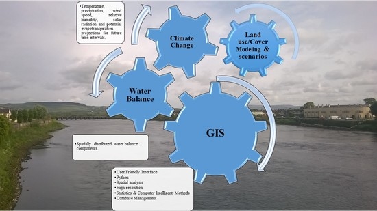
2.1. The Conceptualisation of GEO-CWB Framework

The main idea behind GEO-CWB is to use different integrated modelling methods such as machine learning, physical representation, and geostatistical modelling in order to simplify the simulation of such a complicated environmental problem. The model simulates three different systems, which are climate, land use, and the hydrological system; these simulations capture the geographical changes in addition to temporal changes from climate and land use on the simulated hydrological system. This integration between all the multi-stage modelling processes for the large catchment gives the GEO-CWB an advantage on the other available models, which are limited to small catchment system without the integration between all the modelling stages. In such models, due to computation and practical issues, it would be impossible to include all the known processes in each system in the computation process. Also, it would be challenging to get the physical model or relationship behind each step in the simulation. This is the reason for the use of statistically based models and machine learning techniques in the design of the developed model.

In GEO-CWB, physical-based models have been used in the simulation of hydrological systems and the calculation of different components of the dynamic water balance such as runoff and subsurface water component. The use of physical-based relationships at this stage (see Figure 1) gives the ability to do the multi-iteration process in the simulation without checking the different assumptions inherent in other techniques (such as the assumption of normality for some statistical-based models). Figure 1 shows the relationship between the main GEO-CWB simulation steps: Climate change, land use, and water balance modelling. It shows how the model deals with the spatial and temporal scales in the simulations, and it illustrates that the machine learning techniques are applied in order to get the fine temporal scale outputs for the hydrological parameters. During the dynamical water balance stage, the model works on a high spatial resolution and a fixed temporal scale, which is a monthly time step, after that the results from the water balance stage with the monthly time step are fed to the machine learning techniques in order to work on the finer temporal scale (daily). As illustrated in Figure 1, statistical-based techniques have been used in the fine-scale resolution downscaling for climate simulations. Statistically based models have been used widely in addressing complicated hydrological problems [25,26,27,28,29]. In the developed framework, statistical-based models and machine learning techniques play a crucial role in the parameters scaling process in both spatial and/or temporal dimensions. GEO-CWB provides the ability to use a series of produced land use/cover scenarios using the cellular automata method [29,30,31,32,33] and spatial regression models over a defined temporal scale. GIS is the platform used to run GEO-CWB. This gives GEO-CWB three main advantages: (i) the ability to work with multidimensional files and phenomena, (ii) the ability to reuse the output from GEO-CWB as inputs for other impact models because of the flexibility with the file formats, and (iii) providing a simple, user-friendly interface for such a complicated tool, so the user does not need to use any coding to complete the simulation process.

2.2. GEO-CWB: The Physical Base and Algorithm Design

For the GEO-CWB design process, an integrated approach was adopted to combine all of the simulation processes. This approach, invented in this study, is named as the Pixelated Cubical Balance Approach (PCBA). The idea behind PCBA is to describe the model as a three-dimensional problem moving within a particular time scale, which turns the problem to multidimensional problem, or a four-dimensional problem. The imaginary model extent can be divided into three-dimensional cubes, each cube can be assumed as a single isolated cell moving in time which can be solved against a particular phenomenon by applying its related baseline and boundary conditions. PCBA divides the model extent to small cubes, the higher the number of cubes, the higher the accuracy, with each small cube having its simulation process, which happens within the same time scale. The PCBA concept is applied in GEO-CWB in order to simplify the multidimensional scale complication problem and to allow the linkage between the physical and statistical-based models.

Every single pixel in the domain in each time step runs through the GEO-CWB designed algorithm (Appendix A (Figure A1) and Appendix B), using the input rasterised datasets, as following:

Land cover: Vegetation area fraction, bare area fraction, impervious area fraction, open water area fraction, rooting depth, leaf area index, minimal stomatal resistance, interception percentage, and vegetation height.
Precipitation.
Potential evapotranspiration.
Wind speed.
Temperature.
Groundwater level.
Soil texture: Porosity, wilting point, field capacity, residual water content, a soil empirical parameter for Evapotranspiration (ET) calculation, plant available water, tension saturated height, and soil evaporation depth.
Slope.
Topography: Digital Elevation Model DEM raster.
Average porosity (as a single value) or average porosity raster.
Runoff coefficients: this table contains the runoff coefficients for each single combination of soil, slope, and land use types.

The use of these parameters in GEO-CWB is illustrated in the subsections below.

The following assumptions were made as part of the development of GEO-CWB:

GEO-CWB does not take into account the bedrock geologies of the catchment, so at the moment, it is not possible to get the absolute groundwater recharge value because the data is not available for the Shannon catchment [34]. GEO-CWB instead uses the recharge caps applied to different geological aquifers, which are available for Ireland. So, the aquifer can only accept up to a maximum amount of water. Anything more than this leads to an increase in the subsurface flow/runoff via shallow subsoil pathways [35,36]. These kinds of caps and levels have lots of variabilities and uncertainties in addition to the fact that they are not mapped or available for the Shannon catchment at both temporal and spatial scales. GEO-CWB calculates the subsurface water component which includes both the subsurface flow and the groundwater recharge. The model separates the two main components, subsurface flow and groundwater recharge, once the spatially distributed data for the recharge caps are available.
The actual evapotranspiration, soil evaporation, and transpiration components for the catchment are calculated based on pre-calculated potential evapotranspiration maps. As the actual evapotranspiration is the summation of some calculated sub-fractions of Potential Evapotranspiration (PET) as illustrated in the GEO-CWB equations illustrated in the next sections. Depending on which fraction of each cell is being modelled, the evapotranspiration could be equal to PET (open water fraction) or fraction of it (bare soil or impervious surface fractions) or just equal to the simulated transpiration (vegetated fraction).
GEO-CWB calculates evapotranspiration and interception components individually, which means that the total water loss from precipitation in the catchment is the summation of the two components. A summary of the GEO-CWB assumptions and limitations is provided in Table 1.

2.2.1. GEO-CWB Calculation Stages

In order to parameterise the hydrological response of a catchment to the changes in climate and land use, GEO-CWB has several simulation stages as follows:

2.2.2. GEO-CWB-Stage (1)—Dynamical Water Balance

As illustrated in the previous section, GEO-CWB divides the model domain into pixels and then runs the simulation for each pixel, so each calculation step has to be run for every single pixel. Figure 2 shows the GEO-CWB single-cell water balance components.

In this stage of GEO-CWB, individual dynamical pixel water balance is calculated by summing up the independent pixel’s subdivision simulated water balance. Depending on the land use type assigned to each pixel, GEO-CWB divides the upper pixel’s surface, into the vegetated area, bare soil area, open- water bodies, and impervious area. The dynamic water balance parameters, which were used in the first stage of the framework, are listed with the assumptions associated with them.

The water balance components of vegetated, bare-soil, open-water, and impervious surfaces were used to calculate the total water balance of a raster cell. A precipitation event was taken as a starting point for the computation of the water balance of each of the above-mentioned components of a raster cell, the rest of the processes (runoff, interception, evapotranspiration, and recharge) follow in an orderly manner, see Appendix A (Equation (35)–Equation (38)). This order became a prerequisite for the dynamical monthly time scale within which the processes will be quantified. Appendix A shows the flowchart for the dynamic water balance simulation stage; the flowchart shows that for every single pixel in the model extent, GEO-CWB divides and carries out the pixel simulation, as defined in the following sections.

As illustrated in the flowchart, Appendix A, GEO-CWB divided the modelled area into pixels (50 m by 50 m in the Shannon case study), and then it divided each pixel into fractions (vegetated, open water, bare soil, and impervious surface) each fraction is moving in the time frame (has a temporal dimension). Modelling the water balance using the baseline data and the boundary conditions for every single fraction can be done in a simple and fast way: Each fraction was solved separately and then all the fractions were merged for a single pixel. After running the described simulation for each pixel in the model extent, using all the time steps within the defined temporal dimension, GEO-CWB can then process the large catchment dynamical water balance.

The water balance for a vegetated area depends on the mean seasonal precipitation, interception fraction, surface runoff, actual transpiration, and groundwater recharge. The equations are detailed in Appendix B (Equation (1)–Equation (42)).

Depending on the type of vegetation, the interception fraction represents a constant percentage of the annual precipitation value. Thus, the fraction decreases with an increase in an annual total rainfall amount (since the vegetation cover is assumed to be constant throughout the simulation period). Surface runoff was calculated based on precipitation amount, precipitation intensity, interception, and soil infiltration capacities, using the surface runoff coefficient for vegetated infiltration areas. The surface runoff coefficient is a function of vegetation type, soil type, and slope. Saturated surface runoff occurs in groundwater discharge areas giving rise to a very high surface runoff coefficient. This was due to the reduced dependency on soil, vegetation type, and the vicinity of the area to the river, and was, usually, assumed to be constant. The actual surface runoff is calculated by considering the differences in precipitation intensities and soil infiltration capacities. For example, the coefficient to calculate the actual surface runoff from the potential surface runoff for the groundwater discharge areas is equal to unity since all intensities of precipitation contribute to surface runoff. Only high-intensity storms can generate surface runoff in infiltration areas.

Evapotranspiration depends on which fraction of each cell was being modelled; the evapotranspiration could be equal to PET (open water fraction) or fraction of it (bare soil or impervious surface fractions) or just equal to the simulated transpiration (vegetated fraction). The evapotranspiration calculation depends on the reference value of transpiration, which was obtained from open-water evaporation value and a vegetation coefficient as outlined in the Penman method [38]. The vegetation coefficient can be calculated as the ratio of reference vegetation transpiration to the potential open-water evaporation [38]. For vegetated groundwater discharge areas, the actual transpiration was equal to the reference transpiration as there is no soil or water availability.

The last component, which was the subsurface water component, was then calculated as a residual term of the water balance. This component includes, mainly, a subsurface flow component via shallow pathways and the groundwater recharge component. In general, if the catchment that is being modelled has a shallow sand/gravel aquifer, this subsurface water component will be equal to the groundwater recharge. However, in Ireland a lot of the country is covered in so-called low productivity aquifers where they have an annual recharge cap and the spatially and temporally distributed data for these cap values for the Shannon catchment are not currently available. The spatially distributed subsurface water component was therefore estimated from the vegetation type, soil type, slope, groundwater depth, and climatic variables of precipitation, potential evapotranspiration, temperature, and wind speed. Also, the subsurface water component will be associated with discharge areas, owing to the concept that there was a thin unsaturated zone present even in discharge areas, though this may not have been the case in the summer season. In the summer season, there is high potential transpiration due to vegetation and these result in negative subsurface water component values in discharge areas. In some cases, high winter subsurface water component will compensate for the negative values.

There are two ways of incorporating the change in storage into the model on a seasonal basis. The first was by using different groundwater depth values for winter and summer, while in the second case, the plant available soil moisture reservoir in the winter was assumed to be filled up (i.e., at field capacity) but can be depleted in the summer. A similar procedure to that on vegetated surfaces was followed for the calculation of water balance for bare-soil, open-water, and impervious surfaces. The only difference was that there was no vegetation in these cases, and thus, there were no interception and transpiration terms, see Equation (16)–Equation (34) in Appendix B. To conclude the concepts used in GEO-CWB model in relation to the rainfall-infiltration-runoff computation were based on using a rationale method through actual surface runoff and soil moisture coefficient. Surface runoff was calculated for each pixel and time step using the rational method, which relates runoff peak discharge to rainfall intensity. This was a purely empirical method that correlates peak discharge to catchment characteristics. Once the surface runoff is calculated and the rest of the pixel water balance components were estimated, as discussed above, the only missing component was the subsurface water component which includes infiltration and groundwater recharge and is calculated using the equations in Appendix B.

2.2.3. GEO-CWB-Stage (2)—Surface Runoff Iteration (Calibration Process)

The main aim of this stage was to recalculate the subsurface water component and surface runoff maps by iterating the groundwater depth variable.

The inputs in this stage will be the output from the first stage, and the outputs will be the same variables but after the iteration, all the outputs will have the number two in the file name to indicate that this file was the final map for this parameter, which has resulted from the stage (2).

The main function of this stage was to recalculate the groundwater depth as a response to the simulated subsurface water component and runoff values, then reuse the new groundwater depth values to get the subsurface water component and runoff values; the process was an iteration loop, which stops when the last 10 iterations are equal.

The GEO-CWB calibration process was based on the second stage iteration process of tuning the model based on the measured groundwater levels. The R² for the calibration process after completing the iteration is 79.3%. After the calibration process of the GEO-CWB against the measured groundwater levels in the stage (2) by the iteration process for the surface runoff results, the results of the model need were validated, see Section 3.1. The calibration of the GEO-CWB has shown good results for the simulated parameters, but the model needs further work on developing parameters’ calibration protocol. More parameters had to be taken into account to obtain better results, and surface storage was one of the main settings that needed to be taken into account in the calibration process.

2.2.4. GEO-CWB-Stage (3)—Climate and Land Use Vulnerability Parameters

This stage of GEO-CWB aimed to calculate parameters using the outputs from all the previous stages to assess the vulnerability to climate and land use changes for each climatic period and land use scenario. The calculated parameters were as following:

The accumulated runoff volume in the rainy season was an indication of how much runoff water could be harvested every year during the rainy season.
The safe yield groundwater abstraction rate expressed in (m³/d/ha). GEO-CWB produced groundwater safe yield maps, which estimated how much groundwater can be pumped sustainably without depleting the groundwater resources. Safe yield is usually expressed as a percentage of the groundwater recharge. Several authors from the least conservative 100% to a reasonably conservative 10% have suggested different values [39,40,41]. In general, sustainable yield should be considerably less than the groundwater recharge to sustain both the quantity and quality of streams, springs, wetlands, and groundwater dependent ecosystems [39,40,41]. Based on the different studies reviewed, GEO-CWB adapted the 25% as a sustainable groundwater yield percentage from the calculated subsurface water component. This was a simplistic formula for a country such as Ireland which has such differences in geology and aquifer types, so the results for Shannon were just a good indication for the decision makers.
The water deficit for ideal crop growth (WD) can be estimated as the difference between the crop water requirement and the actual evapotranspiration that was feasible only by rainfall. The crop water requirement can be defined as the amount of water needed to meet the water loss through evapotranspiration for optimal crop growth, which can be estimated as a crop coefficient time’s reference evapotranspiration of well-watered grass [42,43]. Crop coefficients vary between 0.70 and 1.15 depending on crop type and growing stage. The crop coefficient can be assumed to be one and reference evaporation to equal PET, which allows an estimation of how much water was needed for supplementary irrigation for optimal crop growth [44,45]. This calculation can be made on an annual basis, but it was more interesting to do this separately for the summer season, and the winter season, GEO-CWB used Equation (42) in Appendix B, where WD was the water deficit, PET was the potential evapotranspiration, ET was the actual evapotranspiration, and Dn was the number of days in the season.

2.2.5. GEO-CWB-Stage (4)-Statistics Tables

This stage imported all the outputs from all the previous stages and ran spatial statistical algorithms to get the following statistical parameters for each resulted raster file. The results were exported as Excel tables (.csv files).

The frequency
The summation of all the cells
The mean of all cells
The minimum value
The maximum value
The range
The standard deviation
The count of the cell numbers

Table A1 in the appendix shows a summary of the annual, summer, and winter rasters’ areal statistics for all simulated water balance components by GEO-CWB for the baseline period and the projected periods with the calculated average values of the error in the simulated water balance for the case study.

2.2.6. GEO-CWB Integration with GIS

GEO-CWB was fully integrated into the GIS platform; the model is a geospatial multi-dimensional model written in Python and uses ArcMap from ESRI as a running environment. GEO-CWB has a friendly interface integrated into the ArcMap toolbox, which means that the user does not need to use any coding to run the model. The user interfaces for GEO-CWB are presented in Appendix C (Figure A1, Figure A2, Figure A3, Figure A4 and Figure A5).

2.3. GEO-CWB Application: Climate and Land Use Changes Effects on the Shannon River Catchment

This section provides the results of applying GEO-CWB on the Shannon catchment in Ireland as an example of a large and complicated hydrological system. This study shows the simulated and projected annual, winter, and summer average raster maps and results for the GEO-CWB outputs for each land use and climate change scenario for the baseline period and the three projected periods 2020, 2050, and 2080. The baseline period is defined as the long-term average raster data from 1961 to 2000. This section also shows the validation process for the GEO-CWB simulations.

2.4. Data Setup and Study Area

This study presents the primary results of the calculated PETS for both the baseline period and the future periods, based on climate change projections, for the Shannon River catchment in Ireland [13,32,46,47,48,49]. The River Shannon catchment, the focus of this study, is the largest transboundary river system and catchment in the island of Ireland and one of the most important water and power resources in the Republic of Ireland, see Figure 3.

In this study, GEO-CWB simulated different scenarios based on the different inputs scenarios of climate, potential evapotranspiration, and land use scenarios simulated by [32,46,47,49]. The GEO-CWB inputs in this study are listed as follows:

Land cover scenarios simulated by [32].
Precipitation simulated by [49].
Potential evapotranspiration simulated by [46].
Wind speed simulated by [49].
Temperature simulated by [49].
Groundwater level obtained from Geological Survey Ireland (GSI).
Soil texture obtained from GSI.
Slope obtained from NASA’s Shuttle Radar Topography Mission (SRTM).
Topography (DEM raster) obtained from NASA’s SRTM.
Average porosity derived from data collected by GSI.
River flow and levels data which were obtained from Irish Environmental Protection Agency (EPA), Office of Public Works (OPW), and Electricity Supply Board (ESB).

Regarding the land cover/use scenarios, in this study, GEO-CWB used four different land cover scenarios baselines, 2020, 2050, and 2080 obtained from [32]. Gharbia et al. [32] showed that the Shannon Basin area indicated an increase of urban area around 1.75% in 2020 from the baseline, which is a total of 28.53 km² of land will be converted into urban areas in 2020. The simulated increase of urban area in 2050 was around 2.34%, which is a total of 136.38 km² of land will be converted into urban areas in 2050. However, the simulations showed that the Shannon Basin area indicated an increase of the urban area of 2.92% in 2080, which is a total of 244.05 km² of land will be converted into urban areas in 2080. That means the overall urban change percentage from baseline scenario to 2080 will be 83.37%. Most of the urban area will come from the conversion of agricultural to urban areas; also, a small portion of the increase will be from converting wetlands and forest to an urban area. Climatic variables and scenarios were adapted from [47,49]. In addition to the baseline period, climate change projections for the Shannon River Basin District were obtained from multi Global Climate Model (GCM) ensembles for three future time intervals (2020, 2050, and 2080) using a range of different representative concentration pathways (RCPs). The climate change models were based upon two different RCPs; using a radiative forcing of 4.5 W/m² and 8.5 W/m², respectively, which were produced from 50% (median) and 75% (3rd quartile) multi-GCM ensembles results.

In general, Gharbia et al. [49] simulations results show that temperature will increase every year, in particular, RCP 8.5 (75%) has the highest increasing rate (1.85 °C in 2080 as an average over Shannon catchment), which is consistent with the global rise in air temperatures. Gharbia et al. [49] concluded that all seasons would have an increase in temperature with the highest increases occurring in the spring and summer. Trends in precipitation show greater regional variation than temperatures, with occasional conflicting trends from stations which are geographically relatively close. However, there is evidence of an increase in the quantity of precipitation with time in general, except for RCP 4.5 (50%) values, they are higher in 2050 than 2080 and that because of the different adapted parameters in the downscaled GCMs in that particular climate scenario. Gharbia et al. [49] show that RCP 8.5 (75%) would predict the highest future precipitation quantities over the catchment. Gharbia et al. [49] provide multidimensional climatological datasets and simulations for the Shannon River catchment based on four future scenarios RCP4.5(50%), RCP4.5(75%), RCP8.5(50%), and RCP8.5(75%). The same scenarios were developed for potential evapotranspiration by [46], and they have been used in his study as input from the GEO-CWB.

3. Results and Discussion

3.1. GEO-CWB Validation

After the calibration process of the GEO-CWB against the measured groundwater levels in the stage (2) by the iteration process for the surface runoff results, the results of the model need to be validated. The spatial scale used in the application of GEO-CWB on the Shannon River catchment was 50m and the temporal scale was daily time steps. The results of the GEO-CWB model are validated against river flow observations for selected hydrometric stations for the Shannon River catchment, see Figure 4. The river flow data was collected by the Irish EPA, OPW, and ESB data which are available as daily values covering the period from 1972 to 2014. Accumulated monthly river flows were calculated and then accumulated to annual flows at the seven gauging stations, representing the main sub-catchments, then the average daily values got calculated, as shown in Table 2. In order to estimate the annual river discharge at the river gauging stations from the GEO-CWB results, surface runoff and subsurface water component, which includes subsurface water flow and groundwater recharge, were accumulated based on topography for the baseline period simulation, see Figure 5. Because surface runoff flows downgradient, it was possible to calculate the accumulated surface runoff at each point in the basin, using the standard hydrology GIS toolbox. The accumulated surface runoff represents the direct river flow. For the baseflow, it follows from the groundwater balance that long-term average drainage of groundwater should equal the groundwater recharge minus possible groundwater abstractions such as pumping wells. The groundwater abstraction can be ignored in the Shannon river catchment because most of the water consumption was taken from the surface water and any wells are only domestic with very small pumping rates compared to the total recharge [50].

The relationships between areas where groundwater recharge and discharge are occurring depend upon the groundwater flow system in the catchment, which is largely unknown and complicated in the Shannon River catchment. Groundwater flow systems are often strongly conditioned by topography [51,52,53,54]. As an approximation, it was assumed that the groundwater flow was also influenced by topography and river baseflow could be estimated by accumulating the GEO-CWB calculated subsurface water component, which includes subsurface flow and groundwater recharge, on the basis of topography as was done for surface runoff. The accumulated GEO-CWB surface runoff and subsurface water component at the locations of the hydrometric stations were calculated, then the average daily simulated water flow has been calculated and compared with the observed daily average flows in Table 2. The model results are close to the observations with an average percent of error around 5% and the standard deviation for the validation is around 2.13 m³/s with an R² 98.3%. The maximum error percentage (33.88%) was associated with the Nenagh hydrometric station and that was mainly because it was a relatively small catchment with short retention time. The results of the validation process indicated that GEO-CWB simulated the water balance to a high level of accuracy. Table A1 in the appendix shows a summary of the annual, summer, and winter rasters’ areal statistics including the error values in the simulated water balance for the Shannon River case study.

3.2. Water Balance Simulated Parameters Results and Discussions

This section shows the simulated annual, summer, and winter water balance variables and components for the Shannon River catchment by GEO-CWB model forced by the simulated climate change scenarios, land use scenarios, and the simulated PET scenarios.

3.2.1. Surface Runoff

The annual average surface runoff maps simulated by GEO-CWB are shown in Figure 6. The runoff simulations and projections were presented for the baseline period and four climatic scenarios, which were RCP 4.5 50%, RCP 4.5 75% RCP 8.5 50%, and RCP 8.5 75%, projected for three future time steps 2020, 2050, and 2080. The overall statistics for the surface runoff simulations are presented in Appendix D (Table A1), which show that, in general, the annual simulated surface runoff values vary through the climate change scenarios between the positive changes from the baseline and the negative changes from the baseline, as shown in Figure 6. Most of the changes in runoff were negative changes except for 2050 and 2080 of RCP 8.5 (75%) scenario, as the precipitation has a significant increase based on this climate scenario.

The largest surface runoff occured on the rock soil group with wetlands, while the lowest values were for Luisol soil group with agricultural areas. The traceability of the soil type boundaries and the higher standard deviation values of the runoff for different soil groups indicated that surface runoff was more influenced by soil type than by land-use.

Studying the different runoff values based on different soil profiles interactions with land use categories was very important in deriving conclusions about which land use category combined by which soil group gives the lowest or the highest runoff values. That helps in the designing process of structures like rainwater collection basin, landfill, or wastewater plants. The simulations showed that urban areas seem to have lower runoff values for some of the soil groups except groundwater gley, rendzina soil, brown earth, and rock. This was mainly because most of the urban areas in the Shannon catchment were placed on top of relatively permeable soil groups which helped in increasing the infiltration process and that decrease the surface runoff. One can notice that there were wide variations of runoff values over the water bodies. These variations were mainly because of the different type of water body bed soil group and if there is any vegetation in it or not.

3.2.2. Subsurface Water Component

Groundwater recharge is concerned with the percolation of water through the soil, subsoil, and down through the unsaturated zone to the water table [50]. In general, groundwater recharge is estimated by first calculating the effective rainfall (defined as total rainfall minus actual evapotranspiration) through a soil moisture deficit method and then multiplying the calculated effective rainfall by a recharge coefficient [34,50,55,56,57]. The recharge coefficient is the percent of the effective rainfall that forms the groundwater recharge. The recharge coefficient depends mainly on the characteristics of the superficial deposits that overlie the aquifer. Where an aquifer is covered by thick glacial tills of low hydraulic conductivity, the recharge coefficient will be low, with most the effective rainfall being ‘lost’ to surface runoff or interflow.

On the other hand, the recharge coefficient will be high where the overburden is thin, absent, or has high hydraulic conductivity [56]. Misstear et al. [34] stated that there is a clear relationship between recharge coefficient and groundwater vulnerability, with high recharge coefficients expected in highly vulnerable aquifers and so on, based on that, Misstear et al. [34] developed a methodology for making initial estimates of groundwater recharge from groundwater vulnerability mapping. However, the developed methodology gives a good starting estimation, but it is not enough to use its results for any management of the modelling approach. GEO-CWB provides the framework of a cell by cell multidimensional dynamical groundwater recharge calculation for the catchment scale by applying the water balance calculation for each cell’s subfraction, which provides a high accuracy simulation compared with the currently used approaches, when the spatially distributed recharge caps data is available.

Based on the fact that, currently, GEO-CWB does not take into account the bedrock geologies of the catchment and, also, the spatially distributed recharge caps data is not available, GEO-CWB provides as one of the main outputs the sub-surface water component, which includes mainly the subsurface water flow and the groundwater recharge. Groundwater recharge in the Shannon River catchment basin, and anywhere else is promoted by low evapotranspiration and low surface runoff, e.g., typically for a flat topography and permeable soils. The annual averages of the spatially distributed subsurface water component, subsurface flow and groundwater recharge, maps for baseline period and the three projected periods, 2020, 2050, and 2080, forced by four different climatic scenarios are shown in Appendix D (Figure A7).

The simulated annual subsurface water component values vary through the climate change scenarios between 1% to 9% positive increasing changes from the baseline (see Figure 5), this was because the RCP models are predicting higher rainfall quantities which offset the ET, see Figure 7. The annual subsurface water component in the Shannon River catchment is estimated as 40%–55% of the total annual precipitation over the catchment. In general, around 84% of the contribution in the subsurface water component during the 6 months’ rainy season in the winter while the remaining 16% occurs in the 6 months’ summer season. The largest subsurface water component was observed for the agricultural area on Podzol soil. This was basically because of the high permeability of these soils but could partly also be due to lower evaporation rates and less runoff on the relatively gentler slopes of agricultural lands.

3.2.3. Rainfall Interception

Rainfall interception is the fraction of precipitation which falls onto vegetation but never reaches the ground. Instead, it evaporates from the wet canopy. The most direct way to measure rainfall interception evaporation is through the construction of weighing lysimeters, which is a major undertaking for forests [58]. Therefore interception loss (the amount of rainfall lost to wet canopy evaporation) has usually been derived as the residual between event gross precipitation measured above the canopy or in a nearby clearing, and net precipitation, the latter calculated as the sum of separately measured through fall and streamflow below the canopy [2]. GEO-CWB calculates the interception as a direct fraction of precipitation, separated from the evapotranspiration, which means the total water loss from the precipitation in the catchment can be calculated by the summation of both evapotranspiration and interception. The annual spatially distributed interception maps for the baseline period and the three projected periods, 2020, 2050, and 2080, forced by four different climatic scenarios are shown in Appendix D (Figure A8).

As shown in Figure 8, the simulated annual interception values vary through the climate change scenarios between 0.1% to 9% positive increasing changes from the baseline, Figure 5. The annual rainfall interception in the Shannon River catchment makes around 11% of the total annual precipitation over the catchment. In general, around 65% of the interception occurs during the 6 months’ summer season while the remaining 35% occurs in the 6 months’ winter season.

3.2.4. Evapotranspiration

Evapotranspiration was calculated in the GEO-CWB as the sum of transpiration, and evaporation from open water bodies and soil. The actual evapotranspiration was a summation of some calculated sub-fractions of PET as illustrated in the equations in Appendix B. Depending on which fraction of each cell was being modelled, the evapotranspiration could be equal to PET (open water fraction) or fraction of it (bare soil or impervious surface fractions) or just equal to the simulated transpiration (vegetated fraction). GEO-CWB calculates evapotranspiration and interception components individually, which means that the total water loss from precipitation in the catchment was the summation of the two components.

The annual averages spatially distributed evapotranspiration maps for the baseline period and the three projected periods, 2020, 2050, and 2080, forced by the four different climatic scenarios are shown in Appendix D (Figure A9).

The maximum annual evapotranspiration in the catchment is potential evapotranspiration from open water. Evapotranspiration and interception together were estimated to be around 30%-40% of the annual precipitation in the Shannon River catchment. Around 76% of the evapotranspiration takes place during the summer season, while the remaining 24% takes place during the winter season, which was obviously due to the unequal temporal distribution of the temperature but also partly to the fact that the vegetation was less active in the winter season.

It can be noticed that evapotranspiration of the catchment was heavily influenced by soil type. The evapotranspiration maps areal statistics are presented in Appendix D (Table A1), which shows that, in general, the annual simulated evapotranspiration values vary through the climate change scenarios between the positive changes from the baseline and the negative changes from the baseline, (see Figure 9). The mean annual evapotranspiration for different land uses categories showed that urban areas had the lowest values. While overall evapotranspiration was highly influenced by precipitation and to some extent by soil texture, the standard deviation values in Table A1 show that evapotranspiration in the Shannon River catchment was more variable within land-use categories than within soil group.

3.2.5. Soil Evaporation

Soil evaporation was the evaporation from an open soil area as a fraction of each simulated pixel and forms a part of the total evapotranspiration. The annual averages spatially distributed soil evaporation maps for the baseline period and the three projected periods, 2020, 2050, and 2080, forced by the four different climatic scenarios are shown in Appendix D (Figure A10).

The soil evaporation maps areal statistics are presented in Table A1, which show that, in general, the annual simulated soil evaporation has positive changes from the baseline (see Figure 10). As the precipitation increases through all the climatic scenarios, the soil moisture increases as well, which means more water was available for the evaporation process and, thus, the temperature increases. This led to a positive increase in the soil moisture among all the climatic periods and scenarios, as shown in Figure 10 compared to the baseline soil evaporation values, see Figure 5.

3.2.6. Transpiration

Transpiration was the vaporisation of water which was contained in plant tissues, that mainly occurs through the stem and leaf stomata. Transpiration, like direct evaporation, depends on factors such as radiation, air temperature, air humidity, and wind speed. Also, the soil water content and the ability of the soil to conduct water upwards play a role. The length of the plant’s root system also plays an important role in determining the transpiration rate, in addition to the vegetation type. The annual spatially distributed average transpiration maps for the baseline period and the three projected periods, 2020, 2050, and 2080, forced by the four different climatic scenarios are shown in Appendix D (Figure A11). The transpiration maps areal statistics are presented in Table A1, which show that, in general, the annual simulated transpiration varies between positive and negative changes from the baseline, based on the different simulated climatic scenarios (see Figure 11). As RCP8.5 (75%) has the highest increase in temperature and solar radiation, in addition to the predicted increase in the vegetation cover by 2080, the climatic period 2080 has the highest increase in transpiration as shown in Figure 11 compared with the baseline period transpiration, see Figure 5. The average baseline transpiration is around 30 mm/year, and the highest increase related to RCP 8.5 (75%) was about 8.2% in 2080 which is equal to 2.5 mm/year, this amount of increase is very little in term of quantity.

3.2.7. Error in Water Balance/Change in Storage

GEO-CWB calculates the error/change in storage fraction in each simulated cell water balance, which provides an error/change in storage in water balance map for each simulated time step in each simulated climatic scenario. The small error/change in storage in the water balance comes from the assumption that water bodies can always evaporate at the PET rate. Hence, this error should be subtracted from the runoff as open water bodies are supplied by runoff from surrounding areas, and it does not leave the basin as river flow but is evaporated instead. The annual spatially distributed average error in water balance maps for baseline period and the three projected periods, 2020, 2050, and 2080, forced by the four different climatic scenarios are shown in Appendix D (Figure A12). However, the average simulated error in water balance for each climatic period can be shown in Figure 12.

3.2.8. Simulated and Projected Water Balance for Shannon Catchment

The water balance simulation was based upon the continuity equation, i.e., inflow equals outflow plus the storage. Precipitation was the most significant inflow component. The most important outflow components of water balance were surface runoff, evapotranspiration, and subsurface water component, which includes groundwater recharge and subsurface runoff. Any simulated area that receives higher precipitation than the amount of water that it loses has a water surplus. However, regions with a water deficit would get a smaller amount of rainfall than the amount that they lost through evapotranspiration.

Summaries of the numerical contributions to this net balance of the various components, which were discussed earlier in this study are presented in Figure 13, based on the simulated climatic scenarios for each projected period. The overall summary of the water balance of the Shannon River catchment is given in Appendix D (Table A1).

3.2.9. Vulnerability Parameters Results

GEO-CWB produces some parameters from which an assessment can be made of the vulnerability to climate and land use changes for each climatic period and land use scenario, as follows.

Accumulated Surface Runoff Volume

The accumulated runoff volume in the winter season was an indication of how much runoff water could be harvested every year during the winter. Figure A13, in Appendix D, shows the calculated accumulated runoff volume as results of the different climate change conditions and land use scenarios. For the illustrated annual accumulated runoff, the baseline annual areal average accumulated runoff was 14.59 × 10⁶ m³ as an average for all cells in the simulation domain. However, the areal average value for the accumulated runoff for the climatic period the 2080s forced by RCP 8.5 (75%) climatic scenario was 15.48 × 10⁶ m³, which means the average increase in the accumulated runoff was around 6%. However, the areal accumulated runoff average for the whole catchment was increased, but hotspot areas spatial distribution is changed as results of climate and land use changes.

The Safe Yield Groundwater Abstraction

The safe yield groundwater abstraction rates expressed in (m³/d/ha) calculated by GEO-CWB were simplification values for such a large catchment like Shannon, which can only be used as an indication and a rough estimate for how much groundwater can be abstracted in a sustainable way without depleting the groundwater resources. Figure A14, in Appendix D, shows the annual and seasonal calculated safe yield groundwater abstraction volume as results to the different climate change conditions and land use scenarios.

The Water Deficit for Ideal Crop

The water deficit for ideal crop growth, which can be estimated as the difference between the crop water requirement and the actual evapotranspiration. In the Shannon River catchment, most of the catchment was covered in grass (pasture), and there was hardly any deficit, which one can observe.

4. Conclusions

Parameterising the spatially distributed dynamic catchment water balance was a key factor in studying the hydrological system responses to climate and land use changes. This research study presents a developed GIS-based algorithm, which was designed, based, on integrated physical, statistical, and machine learning algorithms. GEO-CWB has been applied on the Shannon catchment in Ireland as an example of a large and complex hydrological system. The results of the GEO-CWB model were validated against river flow observations for seven hydrometric stations for the Shannon River catchment. The model results were close to the observations with an average percent of error around 5%, and the standard deviation for the validation was around 2.13 m³/s and the R² is 98.3%. The results of the validation process indicated that GEO-CWB simulates the water balance with high accuracy. This study shows the simulated annual, summer, and winter water balance variables and components for the Shannon River catchment by the GEO-CWB model forced by the simulated climate change scenarios, land use scenarios, and the simulated PET scenarios. The water balance simulations and projections are presented for the baseline period (1961-2000) and four climatic scenarios, which are RCP 4.5 50%, RCP 4.5 75%, RCP 8.5 50%, and RCP 8.5 75%, projected for three future time steps 2020, 2050, and 2080. The results show that the largest surface runoff occured on the rock soil group with wetlands, while the lowest values were for Luisol soil group with agricultural areas, and the traceability of the soil type boundaries and the higher standard deviation values of the runoff for different soil groups indicate that Shannon’s surface runoff was more influenced by soil type than by land-use. GEO-CWB provides cell by cell multidimensional dynamic subsurface water component values, which include groundwater recharge and subsurface runoff, for the catchment scale by applying the water balance calculation for each cell’s subfraction, which provides a high accuracy simulation compared with the currently used approaches. The simulated annual subsurface water component values vary through the climate change scenarios between 1% to 9% positive increasing changes from the baseline. In general, around 84% of the subsurface water component contribution occurs during the 6 months of the winter season while the remaining 16% occurs in the 6 months’ summer season. The largest subsurface water component was observed for the agricultural area on Podzol soils. This was attributed to the high permeability of these soils but could partly also be due to lower evaporation rates and less runoff on the relatively gentler slopes of agricultural lands. The simulated annual interception values vary through the climate change scenarios between 0.1% to 9% positive increasing changes from the baseline. The annual rainfall interception in the Shannon River catchment makes around 11% of the total annual precipitation over the catchment. In general, around 65% of the interception occurs during the 6 months’ winter season while the remaining 35% occurs in the 6 months’ summer season. The maximum annual evapotranspiration in the catchment was potential evapotranspiration from open water. Evapotranspiration and interception together can be estimated to around 30%-40% of the annual precipitation in the Shannon River catchment. Around 76% of the evapotranspiration takes place during the summer season, while the remaining 24% takes place during the winter season, which was obviously due to the unequal temporal distribution of the temperature but also partly to the fact that the vegetation was less active in the winter season. In general, the annual simulated evapotranspiration values vary through the climate change scenarios between the positive changes from the baseline and the negative changes from the baseline. The mean annual evapotranspiration for different land uses categories showed that urban areas have the lowest values. While the overall evapotranspiration was highly influenced by precipitation and to some extent by soil texture, the standard deviation values show that evapotranspiration in the Shannon River catchment is more variable within land-use categories than within soil group. GEO-CWB produces some calculated parameters to assess the vulnerability to climate and land use changes for each climatic period and land use scenario. These parameters are the accumulated surface runoff volume, the safe yield groundwater abstraction rate, and the water deficit for ideal crop growth. For example, the baseline annual areal average accumulated runoff was 14.59 × 10⁶ m³ as an average for all cells in the simulation domain, however, the areal average value for the accumulated runoff for the climatic period the 2080s forced by RCP 8.5 (75%) climatic scenario was 15.48 × 10⁶ m³, which means the average increase in the accumulated runoff was around 6%. However, the areal accumulated runoff average for the whole catchment is increased, but hotspot areas spatial distribution is changed as a result of climate and land use changes.

GWO-CWB has some critical assumptions and limitations. GEO-CWB does not take into account the bedrock geologies of the catchment. Thus, it provides as one of the main outputs of the sub-surface water component, which includes mainly the subsurface water flow and the groundwater recharge. Also, GEO-CWB does not use the physical basis for the routing process in order to calculate the water flow. It has the unique application of using the machine learning techniques to estimate the flows, so there is potential to develop a technique with integrates the physics and the machine learning techniques to calculate flows as part of GEO-CWB. The application of the GEO-CWB has shown good results for the simulated parameters, but the model needs further work on developing parameters’ calibration protocol. More parameters have to be taken into account to obtain better results, and surface storage is one of the main settings that need to be taken into account in the calibration process.

Author Contributions

Conceptualization, S.S.G.; Methodology, S.S.G., L.G. and F.P.; Software, S.S.G.; Validation, S.S.G., L.G., P.J.; Formal analysis, S.S.G.; Investigation, S.S.G.; Resources, F.P.; Data curation, S.S.G.; Writing—Original draft preparation, S.S.G.; Writing—Review and editing, all authors.; Visualization, S.S.G.; Supervision, F.P.; Project administration, F.P. and L.G.; Funding acquisition, F.P. All authors have read and agreed to the published version of the manuscript.

Funding

This research was funded jointly by Trinity College, Dublin through the Postgraduate Ussher Fellowship Award and by iSCAPE (Improving Smart Control of Air Pollution in Europe) project, which is funded by the European Community’s H2020 Programme (H2020-SC5-04-2015) under the Grant Agreement No. 689954.

Conflicts of Interest

The authors declare no conflict of interest.

Appendix A. GEO-CWB Cell-by-Cell Calculations Flow Chart

Figure A1. GEO-CWB cell-by-cell calculations flow chart.

Appendix B. GEO-CWB Main Equations

Equations’ Parameters and abbreviations:

F_v:	Vegetated fraction
F_ow:	Open water
F_bs:	bare soil fraction
F_is:	Impervious surface fraction
P:	Precipitation
I:	Interception
S_v:	Surface runoff in the vegetated fraction
T_v:	Transpiration
T_rv:	Reference transpiration
E_o:	Seasonal potential evapotranspiration
S_r:	Potential surface runoff
C:	Vegetation coefficient
T:	Temperature
H:	Vegetation height
h_w:	Wind measuring height
U:	Wind speed (Km/hr)
Gwd:	Groundwater depth
R_d:	Rood depth
h_t:	Tension saturated height
PWA:	Plant available water content
a:	Calibrated soil texture factor [59]
Eps:	Penman evaporation for wet soil
S_o:	Runoff of open water fraction
R_o:	subsurface water of open water fraction
Pet:	Potential evapotranspiration
R_cell:	The cell subsurface water component

Interception= F_{(function of land use/cover)} × P

(1)

Potential surface runoff (Ro_(PO))= F_{(vg,so,sl,wd)} × (p − I)

(2)

Final surface runoff = F_{(Intensity, infiltration rate, wd)} × Ro_(PO)

(3)

R_a = Ln( (hw − 0.499H)/(0.123H))/(0.16 U × 0278)

(4)

When H_{(vegetation height )} < 0.15 m, LAI = 24 × H

(5)

When H_{(vegetation height )} > 0.15 m, LAI = 1.5 Ln (H) + 5.5

(6)

R_c = 100/(0.5 × LAI)

(7)

γ/Δ = 1.5411 e^(−0.057 × Temperature)

(8)

C _{(vegetation coefficient)} = (1 + γ/Δ)/(1 + γ/Δ × (1 + (Rc/Ra))

(9)

Trv _{(reference transpiration)} = C × Pet

(10)

When Gwd > Rd + ht, W = P + n × (PAW) × Rd

(11)

F(PAW) = 1 − A^(W/T_rv)

(12)

Transpiration = F (PAW) × T_rv

(13)

When Gwd < Rd + ht

(14)

Transpiration in vegetated groundwater discharge areas = Trv

(15)

Subsurface water for vegetated fraction = P − Interception − Vegetated surface runoff − Transpiration

(16)

Open Water Fraction (Fow)

Interception = F_{(function of land use/cover)} × P = 0

(17)

Final surface runoff = 1 × (P − I)

(18)

T_v = 0.00

(19)

Open water evaporation = 1 × Pet

(20)

Open water subsurface water = P − E_ow − S_ow

(21)

Bare Soil Fraction (Fbs)

Interception = F_{(function of land use/cover and soil texture)} × P

(22)

Potential surface runoff = F_{(vg,so,sl,wd)} × (p − I)

(23)

Final surface runoff = F_{(Intensity, infiltration rate, wd)} × Ro_(po)

(24)

Final surface runoff = F_{(Intensity, infiltration rate, wd)} × Ro_(po)

(25)

W = P + n × (PAW) × Rd

(26)

Eps (Penman evaporation rate for wet soil) = F (function of water content at field capacity and at root zoon, welting point)

(27)

F (PAW) = 1 − A^(W/Eps)

(28)

Soil evaporation = F (PAW) × Pet

(29)

Bare soil subsurface water = P − soil runoff − soil evaporation

(30)

Impervious surface fraction (Fis)

Interception = F_{(function of land use/cover)} × P

(31)

Potential surface runoff = F_{(lu,so,sl,wd)} × (p − I)

(32)

Final surface runoff = F_{(Intensity, infiltration rate, wd)} × Ro_(po)

(33)

Fie = F_{(Impervious surface evaporation fraction a function of land use type)}

(34)

Impervious surface evaporation = Pet × Fie

(35)

Impervious surface subsurface water component = P − Impervious surface evaporation − Impervious surface runoff

(36)

Pixel/Cell water balance

Et _cell = (F_v × Et_v) + (F_ow × E_ow) + (F_is × E_i) + (F_bs × E_s)

(37)

S _cell = (F_v × S_v) + (F_ow × S_ow) + (F_is × S_i) + (F_bs × S_bs)

(38)

R _cell = (F_v × R_v)+ (R_ow × E_ow )+ (F_is × R_i) + (F_bs × R_s)

(39)

Cell Water Balance:

P _cell = Et _cell + S _cell + R _cell + I _cell

(40)

Error and the change in the storage in pixel water balance

The following equation quantifies the proportional error and the change in the storage per time step in the simulated water balance.

Error in Water Balance = (P _cell − R _cell − Et _cell − S cell)/P _cell

(41)

Climate and Land Use Vulnerability Parameters

Accumulated runoff (m^{3}) = \int_{A}^{} (S u r f a c e r u n o f f) d a \times 10^{- 3}

(42)

Safe yield (m^{3} / day / ha) = 6.85 \times 10^{- 3} \times R e c h a r g e (m m)

(43)

WD (m^{3} / day / ha) = \frac{10 \times (P E T - E T)}{D n}

(44)

Appendix C. GEO-CWB User Interfaces

Figure A2. GEO-CWB as a tool in the ARC toolbox.

Figure A3. GEO-CWB stage (1) interface.

Figure A4. GEO-CWB stage (2) interface.

Figure A5. GEO-CWB stage (3) interface.

Appendix D. GEO-CWB Spatially Distributed Mapped Results

Figure A6. The average annual surface runoff for each climatic period and land use scenario simulated by GEO-CWB.

Figure A7. The average annual subsurface water component for each climatic period and land use scenario simulated by GEO-CWB.

Figure A8. The average annual interception for each climatic period and land use scenario simulated by GEO-CWB.

Figure A9. The average annual evapotranspiration for each climatic period and land use scenario simulated by GEO-CWB.

Figure A10. The average annual soil evaporation for each climatic period and land use scenario simulated by GEO-CWB.

Figure A11. The average annual transpiration for each climatic period and land use scenario simulated by GEO-CWB.

Figure A12. The spatially distributed average annual error/change in storage in water balance (mm/year) for each climatic period and land use scenario simulated by GEO-CWB.

Figure A13. The accumulated surface runoff for each climatic period and land use scenario simulated by GEO-CWB.

Figure A14. The average annual safe yield groundwater abstraction for each climatic period and land use scenario simulated by GEO-CWB.

Table A1. Annual, summer and winter rasters’ areal statistics for all simulated water balance components by GEO-CWB for the baseline period and the projected periods with the calculated average values of the error in the simulated water balance.

Scenario	Period	Component	Annual-Mean	Annual-SD	Summer-Mean	Summer-SD	Winter-Mean	Winter-SD
Baseline Period	1961–2014	Runoff (Ro) mm	271.30	496.61	34.05	99.44	47.73	139.91
		Evapotranspiration (Et) mm	166.37	107.21	126.57	81.69	39.81	25.57
		Interception (In) mm	125.59	142.46	82.09	47.16	43.49	97.57
		Transpiration (Tr) mm	30.63	55.28	23.57	42.48	7.06	12.90
		Soil evaporation (Se) mm	102.29	70.58	77.57	53.48	24.72	17.10
		Subsurface water component (Re) mm	744.90	292.95	248.14	116.48	500.27	180.84
		Precipitation (P) mm	1136.27	224.02	486.22	83.58	650.04	143.10
		Water balance (WB) = P-Ro-Et-Re; mm	−46.30	−	77.46	−	62.23	−
		Error in water balance (WB/P; %)	−4.07	−	15.93	−	9.57	−
RCP 4.5 (50%)	2020	Runoff (Ro) mm	267.25	497.17	31.10	95.72	44.02	135.86
		Evapotranspiration (Et) mm	165.40	106.65	130.38	84.19	35.03	22.52
		Interception (In) mm	126.64	144.18	82.49	47.63	44.14	99.66
		Transpiration (Tr) mm	30.25	55.49	24.05	44.08	6.21	11.51
		Soil evaporation (Se) mm	104.06	71.11	81.81	55.85	22.24	15.27
		Subsurface water component (Re) mm	751.09	291.00	281.44	118.93	532.92	180.11
		Precipitation (P) mm	1137.67	223.67	484.31	83.02	653.37	143.43
		Water balance (WB) = P-Ro-Et-Re; mm	−46.07	−	41.39	−	41.40	−
		Error in water balance (WB/P; %)	−4.05	−	8.55	−	6.34	−
	2050	Runoff (Ro) mm	252.44	502.26	21.46	85.47	28.97	115.74
		Evapotranspiration (Et) mm	159.40	100.55	125.46	79.40	159.40	100.55
		Interception (In) mm	139.73	159.42	92.65	54.54	47.07	107.60
		Transpiration (Tr) mm	30.13	58.04	23.99	46.56	6.15	11.95
		Soil evaporation (Se) mm	109.36	71.99	86.04	56.56	23.32	11.43
		Subsurface water component (Re) mm	812.41	292.70	281.44	118.93	532.92	180.11
		Precipitation (P) mm	1193.54	239.25	525.06	96.41	668.48	144.61
		Water balance (WB) = P-Ro-Et-Re; mm	−30.71	−	96.70	−	−52.81	−
		Error in water balance (WB/P; %)	−2.57	−	18.42	−	−7.90	−
	2080	Runoff (Ro) mm	255.15	505.23	17.87	74.50	27.04	112.85
		Evapotranspiration (Et) mm	159.26	100.00	125.50	78.85	33.97	21.24
		Interception (In) mm	132.78	157.02	83.50	48.72	49.27	110.69
		Transpiration (Tr) mm	30.23	58.10	23.99	46.20	6.22	12.10
		Soil evaporation (Se) mm	110.17	72.58	86.64	57.00	23.53	15.59
		Subsurface water component (Re) mm	780.54	275.63	242.86	102.99	540.57	179.85
		Precipitation (P) mm	1174.86	221.16	470.30	78.75	677.55	145.37
		Water balance (WB) = P-Ro-Et-Re; mm	−20.09	−	84.07	−	75.97	−
		Error in water balance (WB/P; %)	−1.71	−	17.88	−	11.21	−
RCP 4.5 (75%)	2020	Runoff (Ro) mm	267.54	497.54	31.19	95.97	42.94	135.64
		Evapotranspiration (Et) mm	165.44	106.67	130.41	84.21	35.03	22.52
		Interception (In) mm	126.80	144.06	82.75	47.80	44.05	99.38
		Transpiration (Tr) mm	30.59	58.16	24.25	46.11	6.37	12.19
		Soil evaporation (Se) mm	104.06	71.11	81.81	55.85	22.24	15.27
		Subsurface water component (Re) mm	750.40	290.99	256.58	114.34	508.22	180.39
		Precipitation (P) mm	1137.08	223.94	485.67	83.51	651.41	143.17
		Water balance (WB) = P-Ro-Et-Re; mm	−46.30	−	67.49	−	65.22	−
		Error in water balance (WB/P; %)	−4.07	−	13.90	−	10.01	−
	2050	Runoff (Ro) mm	251.07	499.78	19.78	78.93	29.27	116.93
		Evapotranspiration (Et) mm	159.95	100.95	126.10	79.58	33.86	21.35
		Interception (In) mm	132.95	159.13	85.24	49.60	47.71	109.03
		Transpiration (Tr) mm	30.29	55.55	24.08	44.13	6.21	11.52
		Soil evaporation (Se) mm	109.97	72.42	86.51	56.90	23.47	15.53
		Subsurface water component (Re) mm	789.54	283.24	251.52	107.93	540.83	181.64
		Precipitation (P) mm	1160.53	226.42	483.15	83.18	677.38	145.71
		Water balance (WB) = P-Ro-Et-Re; mm	−40.03	−	85.75	−	73.42	−
		Error in water balance (WB/P; %)	−3.45	−	17.75	−	10.84	−
	2080	Runoff (Ro) mm	250.23	498.52	19.25	76.90	29.25	116.94
		Evapotranspiration (Et) mm	161.50	101.86	127.29	80.36	34.22	21.59
		Interception (In) mm	130.61	154.59	82.79	47.82	47.80	109.21
		Transpiration (Tr) mm	29.98	57.80	23.80	45.89	6.19	12.03
		Soil evaporation (Se) mm	111.09	73.13	87.39	57.45	23.70	15.68
		Subsurface water component (Re) mm	779.81	280.36	241.13	104.39	542.03	182.13
		Precipitation (P) mm	1173.33	229.49	481.63	82.99	691.69	149.02
		Water balance (WB) = P-Ro-Et-Re; mm	−18.21	−	93.96	−	86.19	−
		Error in water balance (WB/P; %)	−1.55	−	19.51	−	12.46	−
RCP 8.5 (50%)	2020	Runoff (Ro) mm	267.31	497.26	31.07	95.61	44.06	135.97
		Evapotranspiration (Et) mm	165.72	106.85	130.63	84.35	35.09	22.56
		Interception (In) mm	126.65	144.23	82.44	47.57	44.20	99.79
		Transpiration (Tr) mm	30.91	58.72	24.50	46.54	6.44	12.39
		Soil evaporation (Se) mm	104.25	71.25	81.97	55.96	22.28	15.30
		Subsurface water component (Re) mm	751.22	291.01	245.23	113.83	510.43	180.86
		Precipitation (P) mm	1148.40	221.01	469.49	78.51	678.90	145.49
		Water balance (WB) = P-Ro-Et-Re; mm	−35.85	−	62.56	−	89.32	−
		Error in water balance (WB/P; %)	−3.12	−	13.33	−	13.16	−
	2050	Runoff (Ro) mm	248.62	500.57	18.18	75.77	27.54	114.95
		Evapotranspiration (Et) mm	160.52	100.77	126.44	79.42	34.09	21.43
		Interception (In) mm	135.86	160.86	85.55	50.26	50.30	113.05
		Transpiration (Tr) mm	30.14	58.13	23.88	46.08	6.28	12.19
		Soil evaporation (Se) mm	111.00	73.17	87.26	57.44	23.74	15.73
		Subsurface water component (Re) mm	800.57	281.89	250.47	105.79	552.82	183.27
		Precipitation (P) mm	1137.92	223.58	483.88	82.79	654.09	143.43
		Water balance (WB) = P-Ro-Et-Re; mm	−71.79	−	88.79	−	39.64	−
		Error in water balance (WB/P; %)	−6.31	−	18.35	−	6.06	−
	2080	Runoff (Ro) mm	247.67	499.28	17.07	71.30	28.11	117.33
		Evapotranspiration (Et) mm	167.55	105.22	131.96	82.93	35.60	22.41
		Interception (In) mm	131.58	159.44	80.06	46.32	51.52	115.49
		Transpiration (Tr) mm	30.31	55.59	24.09	44.16	6.22	11.53
		Soil evaporation (Se) mm	115.92	79.37	91.20	59.95	24.73	16.00
		Subsurface water component (Re) mm	788.75	278.67	225.74	97.05	567.92	186.71
		Precipitation (P) mm	1161.69	218.05	451.37	73.34	710.32	148.23
		Water balance (WB) = P-Ro-Et-Re; mm	−42.28	−	76.60	−	78.69	−
		Error in water balance (WB/P; %)	−3.64	−	16.97	−	11.08	−
RCP 8.5 (75%)	2020	Runoff (Ro) mm	267.80	497.98	30.04	95.22	42.46	135.14
		Evapotranspiration (Et) mm	165.76	106.88	130.67	84.37	35.10	22.57
		Interception (In) mm	127.04	144.75	82.71	47.79	44.33	100.08
		Transpiration (Tr) mm	30.35	55.66	24.13	44.22	6.22	11.54
		Soil evaporation (Se) mm	104.25	71.25	81.97	55.96	22.28	15.30
		Subsurface water component (Re) mm	754.03	292.01	246.32	114.30	512.10	181.40
		Precipitation (P) mm	1141.70	224.82	485.55	83.49	656.15	140.97
		Water balance (WB) = P-Ro-Et-Re; mm	−45.89	−	78.52	−	66.49	−
		Error in water balance (WB/P; %)	−4.02	−	16.17	−	10.13	−
	2050	Runoff (Ro) mm	284.54	510.21	47.65	129.97	70.52	191.81
		Evapotranspiration (Et) mm	163.26	102.95	128.72	81.24	34.55	21.79
		Interception (In) mm	133.72	158.41	84.90	49.37	48.82	111.56
		Transpiration (Tr) mm	30.61	59.02	24.22	46.82	6.24	12.32
		Soil evaporation (Se) mm	112.23	73.93	88.31	58.09	23.92	15.84
		Subsurface water component (Re) mm	769.38	312.20	239.64	111.71	531.45	207.82
		Precipitation (P) mm	1175.13	229.75	481.39	82.96	693.73	149.32
		Water balance (WB) = P-Ro-Et-Re; mm	−42.05	−	65.38	−	57.21	−
		Error in water balance (WB/P; %)	−3.58	−	13.58	−	8.25	−
	2080	Runoff (Ro) mm	283.70	511.54	46.63	127.69	74.62	203.68
		Evapotranspiration (Et) mm	171.71	107.81	135.48	85.13	36.28	22.83
		Interception (In) mm	137.99	167.35	84.46	49.56	53.78	120.66
		Transpiration (Tr) mm	33.19	63.05	26.30	50.01	6.93	13.24
		Soil evaporation (Se) mm	118.60	78.23	93.41	61.52	25.20	16.71
		Subsurface water component (Re) mm	796.81	317.32	230.45	108.94	568.42	216.87
		Precipitation (P) mm	1216.77	235.33	475.93	82.05	741.29	156.21
		Water balance (WB) = P-Ro-Et-Re; mm	−35.45	−	63.37	−	61.97	−
		Error in water balance (WB/P; %)	−2.91	−	13.31	−	8.36	−

References

Zhang, L.; Potter, N.; Hickel, K.; Zhang, Y.; Shao, Q. Water balance modeling over variable time scales based on the Budyko framework–Model development and testing. J. Hydrol. 2008, 360, 117–131. [Google Scholar] [CrossRef]
Van Dijk, A.I.; Gash, J.H.; van Gorsel, E.; Blanken, P.D.; Cescatti, A.; Emmel, C.; Gielen, B.; Harman, I.N.; Kiely, G.; Merbold, L. Rainfall interception and the coupled surface water and energy balance. Agric. For. Meteorol. 2015, 214, 402–415. [Google Scholar] [CrossRef] [Green Version]
Tekleab, S.; Uhlenbrook, S.; Mohamed, Y.; Savenije, H.; Temesgen, M.; Wenninger, J. Water balance modeling of Upper Blue Nile catchments using a top-down approach. Hydrol. Earth Syst. Sci. 2011, 15, 2179. [Google Scholar] [CrossRef] [Green Version]
Zhang, S.; Yang, H.; Yang, D.; Jayawardena, A. Quantifying the effect of vegetation change on the regional water balance within the Budyko framework. Geophys. Res. Lett. 2016, 43, 1140–1148. [Google Scholar] [CrossRef]
le Roux, B.; van der Laan, M.; Vahrmeijer, T.; Bristow, K.L.; Annandale, J.G. Establishing and testing a catchment water footprint framework to inform sustainable irrigation water use for an aquifer under stress. Sci. Total Environ. 2017, 599, 1119–1129. [Google Scholar] [CrossRef]
Marhaento, H.; Booij, M.J.; Rientjes, T.; Hoekstra, A.Y. Attribution of changes in the water balance of a tropical catchment to land use change using the SWAT model. Hydrol. Process. 2017, 31, 2029–2040. [Google Scholar] [CrossRef]
Pfister, L.; Martínez-Carreras, N.; Hissler, C.; Klaus, J.; Carrer, G.E.; Stewart, M.K.; McDonnell, J.J. Bedrock geology controls on catchment storage, mixing, and release: A comparative analysis of 16 nested catchments. Hydrol. Process. 2017, 31, 1828–1845. [Google Scholar] [CrossRef] [Green Version]
Staudinger, M.; Stoelzle, M.; Seeger, S.; Seibert, J.; Weiler, M.; Stahl, K. Catchment water storage variation with elevation. Hydrol. Process. 2017, 31, 2000–2015. [Google Scholar] [CrossRef]
Jung, M.; Reichstein, M.; Schwalm, C.R.; Huntingford, C.; Sitch, S.; Ahlström, A.; Arneth, A.; Camps-Valls, G.; Ciais, P.; Friedlingstein, P. Compensatory water effects link yearly global land CO₂ sink changes to temperature. Nature 2017, 541, 516–520. [Google Scholar] [CrossRef] [PubMed] [Green Version]
Fan, J.; Tian, F.; Yang, Y.; Han, S.; Qiu, G. Quantifying the magnitude of the impact of climate change and human activity on runoff decline in Mian River Basin, China. Water Sci. Technol. 2010, 62, 783–791. [Google Scholar] [CrossRef]
Yonghui, Y.; Fei, T. Abrupt change of runoff and its major driving factors in Haihe River Catchment. China. J. Hydrol. 2009, 374, 373–383. [Google Scholar]
Junkermann, W.; Hacker, J.; Lyons, T.; Nair, U. Land use change suppresses precipitation. Atmos. Chem. Phys. 2009, 9, 6531–6539. [Google Scholar] [CrossRef] [Green Version]
Gharbia, S.; Gill, L.; Johnston, P.; Pilla, F. GEO-CWB: A dynamic water balance tool for catchment water management. In Proceedings of the 5th International Multidisciplinary Conference on Hydrology and Ecology (HydroEco2015), Vienna, Austria, 13–16 April 2015. [Google Scholar]
Gharbia, S.S.; Aish, A.; Pilla, F.; Gharbia, A.S. Potential Effects of Climate Change on Groundwater Recharge-a Case Study of the Gaza Strip, Palestine. In Proceedings of the XVth IWRA World Water Congress, Edinburgh, Scotland, 25–29 May 2015. [Google Scholar]
Bonsch, M.; Humpenöder, F.; Popp, A.; Bodirsky, B.; Dietrich, J.P.; Rolinski, S.; Biewald, A.; Lotze-Campen, H.; Weindl, I.; Gerten, D. Trade-offs between land and water requirements for large-scale bioenergy production. Gcb Bioenergy 2016, 8, 11–24. [Google Scholar] [CrossRef]
Wang, R.; Zimmerman, J. Hybrid analysis of blue water consumption and water scarcity implications at the global, national, and basin levels in an increasingly globalized world. Environ. Sci. Technol. 2016, 50, 5143–5153. [Google Scholar] [CrossRef] [PubMed]
Huang, S.; Kumar, R.; Flörke, M.; Yang, T.; Hundecha, Y.; Kraft, P.; Gao, C.; Gelfan, A.; Liersch, S.; Lobanova, A. Evaluation of an ensemble of regional hydrological models in 12 large-scale river basins worldwide. Clim. Chang. 2017, 141, 381–397. [Google Scholar] [CrossRef]
Kauffeldt, A.; Wetterhall, F.; Pappenberger, F.; Salamon, P.; Thielen, J. Technical review of large-scale hydrological models for implementation in operational flood forecasting schemes on continental level. Environ. Model. Softw. 2016, 75, 68–76. [Google Scholar] [CrossRef]
Devia, G.K.; Ganasri, B.; Dwarakish, G. A review on hydrological models. Aquat. Procedia 2015, 4, 1001–1007. [Google Scholar] [CrossRef]
Sorooshian, S.; Duan, Q.; Gupta, V.K. Calibration of Rainfall-Runoff models: Application of global optimization to the Sacramento Soil Moisture Accounting Model. Water Resour. Res. 1993, 29, 1185–1194. [Google Scholar] [CrossRef]
Pontes, P.R.M.; Fan, F.M.; Fleischmann, A.S.; de Paiva, R.C.D.; Buarque, D.C.; Siqueira, V.A.; Jardim, P.F.; Sorribas, M.V.; Collischonn, W. MGB-IPH model for hydrological and hydraulic simulation of large floodplain river systems coupled with open source GIS. Environ. Model. Softw. 2017, 94, 1–20. [Google Scholar] [CrossRef]
Khan, A.; Ghoraba, S.; Arnold, J.G.; Luzio, M. Hydrological modeling of upper Indus Basin and assessment of deltaic ecology. Int. J. Mod. Eng. Res 2014, 4, 73–85. [Google Scholar]
Rahmati, O.; Kornejady, A.; Samadi, M.; Nobre, A.D.; Melesse, A.M. Development of an automated GIS tool for reproducing the HAND terrain model. Environ. Model. Softw. 2018, 102, 1–12. [Google Scholar] [CrossRef]
Sanzana, P.; Gironás, J.; Braud, I.; Branger, F.; Rodriguez, F.; Vargas, X.; Hitschfeld, N.; Muñoz, J.; Vicuña, S.; Mejía, A. A GIS-based urban and peri-urban landscape representation toolbox for hydrological distributed modeling. Environ. Model. Softw. 2017, 91, 168–185. [Google Scholar] [CrossRef] [Green Version]
Akgun, A.; Erkan, O. Landslide susceptibility mapping by geographical information system-based multivariate statistical and deterministic models: In an artificial reservoir area at Northern Turkey. Arab. J. Geosci. 2016, 9, 165. [Google Scholar] [CrossRef]
Müller, M.; Thompson, S. Comparing statistical and process-based flow duration curve models in ungauged basins and changing rain regimes. Earth Syst. Sci. 2016, 20, 669–683. [Google Scholar] [CrossRef] [Green Version]
Daly, C.; Gibson, W.P.; Taylor, G.H.; Johnson, G.L.; Pasteris, P. A knowledge-based approach to the statistical mapping of climate. Clim. Res. 2002, 22, 99–113. [Google Scholar] [CrossRef] [Green Version]
Legates, D.R.; McCabe, G.J., Jr. Evaluating the use of “Goodness-Of-Fit” measures in hydrologic and hydroclimatic model validation. Water Resour. Res. 1999, 35, 233–241. [Google Scholar] [CrossRef]
Wood, A.W.; Leung, L.R.; Sridhar, V.; Lettenmaier, D. Hydrologic implications of dynamical and statistical approaches to downscaling climate model outputs. Clim. Chang. 2004, 62, 189–216. [Google Scholar] [CrossRef]
Ku, C.-A. Incorporating spatial regression model into cellular automata for simulating land use change. Appl. Geogr. 2016, 69, 1–9. [Google Scholar] [CrossRef]
Chen, Y.; Li, X.; Liu, X.; Ai, B.; Li, S. Capturing the varying effects of driving forces over time for the simulation of urban growth by using survival analysis and cellular automata. Landsc. Urban Plan. 2016, 152, 59–71. [Google Scholar] [CrossRef]
Gharbia, S.S.; Abd Alfatah, S.; Gill, L.; Johnston, P.; Pilla, F. Land use scenarios and projections simulation using an integrated GIS cellular automata algorithms. Modeling Earth Syst. Environ. 2016, 2, 151. [Google Scholar] [CrossRef] [Green Version]
Liao, J.; Tang, L.; Shao, G.; Su, X.; Chen, D.; Xu, T. Incorporation of extended neighborhood mechanisms and its impact on urban land-use cellular automata simulations. Environ. Model. Softw. 2016, 75, 163–175. [Google Scholar] [CrossRef] [Green Version]
Misstear, B.; Brown, L.; Daly, D. A methodology for making initial estimates of groundwater recharge from groundwater vulnerability mapping. Hydrogeol. J. 2009, 17, 275–285. [Google Scholar] [CrossRef]
Mockler, E.; Bruen, M. Parameterizing dynamic water quality models in ungauged basins: Issues and solutions. Underst. Freshw. Qual. Probl. A Chang. World 2013, 361, 235–242. [Google Scholar]
O’Brien, R.J.; Misstear, B.D.; Gill, L.W.; Deakin, J.L.; Flynn, R. Developing an integrated hydrograph separation and lumped modelling approach to quantifying hydrological pathways in Irish river catchments. J. Hydrol. 2013, 486, 259–270. [Google Scholar] [CrossRef] [Green Version]
Gharbia, S.S. An Integrated Water Resources, Climate and Land Use Changes Model for Shannon River Catchment; Trinity College Dublin: Dublin, Ireland, 2017. [Google Scholar]
Penman, H.L. Natural evaporation from open water, bare soil and grass. Proc. R. Soc. Lond. Ser. A. Math. Phys. Sci. 1948, 193, 120–145. [Google Scholar]
Voudouris, K. Groundwater balance and safe yield of the coastal aquifer system in NEastern Korinthia, Greece. Appl. Geogr. 2006, 26, 291–311. [Google Scholar] [CrossRef]
Kalf, F.R.; Woolley, D.R. Applicability and methodology of determining sustainable yield in groundwater systems. Hydrogeol. J. 2005, 13, 295–312. [Google Scholar] [CrossRef]
Zhou, Y. A critical review of groundwater budget myth, safe yield and sustainability. J. Hydrol. 2009, 370, 207–213. [Google Scholar] [CrossRef]
Vaux Jr, H.J.; Pruitt, W.O. Crop-water production functions. In Advances in Irrigation; Elsevier: Amsterdam, The Netherlands, 1983; Volume 2, pp. 61–97. [Google Scholar]
Allen, R.G.; Pereira, L.S.; Raes, D.; Smith, M. Crop evapotranspiration-Guidelines for computing crop water requirements-FAO Irrigation and drainage paper 56. Faorome 1998, 300, D05109. [Google Scholar]
Zhang, Y.; Kendy, E.; Qiang, Y.; Changming, L.; Yanjun, S.; Hongyong, S. Effect of soil water deficit on evapotranspiration, crop yield, and water use efficiency in the North China Plain. Agric. Water Manag. 2004, 64, 107–122. [Google Scholar] [CrossRef]
Kendy, E.; Gérard-Marchant, P.; Todd Walter, M.; Zhang, Y.; Liu, C.; Steenhuis, T.S. A soil-water-balance approach to quantify groundwater recharge from irrigated cropland in the North China Plain. Hydrol. Process. 2003, 17, 2011–2031. [Google Scholar] [CrossRef]
Gharbia, S.S.; Smullen, T.; Gill, L.; Johnston, P.; Pilla, F. Spatially distributed potential evapotranspiration modeling and climate projections. Sci. Total Environ. 2018, 633, 571–592. [Google Scholar] [CrossRef] [PubMed]
Gharbia, S.S.; Johnston, P.; Gill, L.; Pilla, F. Using GIS based algorithms for GCMs’ performance evaluation. In Proceedings of the 2016 18th Mediterranean Electrotechnical Conference (MELECON), Lemesos, Cyprus, 18–20 April 2016; pp. 1–6. [Google Scholar]
Gharbia, S.S.; Gill, L.; Johnston, P.; Pilla, F. Trans-boundary European River’s Long-term Changes Analysis for Water Level and Streamflow Regime. In Proceedings of the 42nd IAH Congress (AQUA2015), Rome, Italy, 13–18 September 2015. [Google Scholar]
Gharbia, S.S.; Gill, L.; Johnston, P.; Pilla, F. Multi-GCM ensembles performance for climate projection on a GIS platform. Modeling Earth Syst. Environ. 2016, 2, 102. [Google Scholar] [CrossRef] [Green Version]
Misstear, B.; Brown, L.; Johnston, P. Estimation of groundwater recharge in a major sand and gravel aquifer in Ireland using multiple approaches. Hydrogeol. J. 2009, 17, 693–706. [Google Scholar] [CrossRef]
Gebreyohannes, T.; De Smedt, F.; Walraevens, K.; Gebresilassie, S.; Hussien, A.; Hagos, M.; Amare, K.; Deckers, J.; Gebrehiwot, K. Application of a spatially distributed water balance model for assessing surface water and groundwater resources in the Geba basin, Tigray, Ethiopia. J. Hydrol. 2013, 499, 110–123. [Google Scholar] [CrossRef]
Tóth, J. Gravitational Systems of Groundwater Flow: Theory, Evaluation, Utilization; Cambridge University Press: Cambridge, UK, 2009. [Google Scholar]
Haitjema, H.M.; Mitchell-Bruker, S. Are water tables a subdued replica of the topography? Ground Water 2005, 43, 781–786. [Google Scholar] [CrossRef]
Freeze, R.A.; Cherry, J.A. Groundwater; Prentice-Hall Inc.: Englewood Cliffs, NJ, USA, 1979. [Google Scholar]
Misstear, B.; Brown, L.; Williams, N.H. Groundwater recharge to a fractured limestone aquifer overlain by glacial till in County Monaghan, Ireland. Q. J. Eng. Geol. Hydrogeol. 2008, 41, 465–476. [Google Scholar] [CrossRef]
Fitzsimons, V.P.; Misstear, B.D. Estimating groundwater recharge through tills: A sensitivity analysis of soil moisture budgets and till properties in Ireland. Hydrogeol. J. 2006, 14, 548–561. [Google Scholar] [CrossRef]
Misstear, B.D. Groundwater recharge assessment: A key component of river basin management. In Proceedings of the River Basin Management, Offaly, Ireland, 21 November 2000; pp. 52–59. [Google Scholar]
Dunin, F.; O’Loughlin, E.; Reyenga, W. Interception loss from eucalypt forest: Lysimeter determination of hourly rates for long term evaluation. Hydrol. Process. 1988, 2, 315–329. [Google Scholar] [CrossRef]
Vandewiele, G.; Xu, C.-Y.; Huybrechts, W. Regionalisation of physically-based water balance models in Belgium. Application to ungauged catchments. Water Resour. Manag. 1991, 5, 199–208. [Google Scholar] [CrossRef]

Figure 1. Geographical spatially distributed water balance model (GEO-CWB) general framework.

Figure 2. GEO-CWB single-cell water balance components (adapted from [37]).

Figure 3. Location map for the Shannon River catchment.

Figure 4. Location map for the selected validation hydrometric stations.

Figure 5. Baseline period GEO-CWB simulation results for the Shannon catchment.

Figure 6. Simulated surface runoff changes percent for each climate change scenario from the baseline period.

Figure 7. Simulated subsurface water component (groundwater recharge and subsurface runoff aggregated together) changes percent for each climate change scenario from the baseline period.

Figure 8. Simulated interception changes percent for each climate change scenario from the baseline period.

Figure 9. Simulated evapotranspiration changes percent for each climate change scenario from the baseline period.

Figure 10. Simulated soil evaporation changes percent for each climate change scenario from the baseline period.

Figure 11. Simulated transpiration changes percent for each climate change scenario from the baseline period.

Figure 12. The average error/change in storage in water balance (%) for each climatic period and land use scenario simulated by GEO-CWB.

Figure 13. GEO-CEB simulated water balance (mm/year).

Table 1. Assumptions and limitations that have been used in GEO-CWB related to different water balance component.

Output Parameters	Assumptions/Limitations
Surface Runoff	It represents the direct surface runoff, and it does not include the subsurface runoff (subsurface flow via shallow subsoil pathways)
Subsurface water	This includes many components mainly subsurface flow via shallow pathways and the groundwater recharge component.
Interception	Based on the vegetation type interception fraction represents a constant percentage of the annual precipitation value, which is the main part of the total water loss in the catchment.
Evapotranspiration	Depending on which fraction of each cell is being modelled, the evapotranspiration could be equal to PET (open water fraction) or fraction of it (bare soil or impervious surface fractions) or just equal to the simulated transpiration (vegetated fraction).
Soil evaporation	Based on the soil type, soil evaporation is a fraction of the PET.
Transpiration	Based on the vegetation type, root depth, groundwater level, soil moisture, tension saturated height, temperature, and many other factors, transpiration is calculated for the vegetated fraction of each cell.

Table 2. GEO-CWB evaluation table between the simulated average daily flow and the observed average daily flow for the simplified Shannon system.

Hydrometric Stations	Simulated Average Daily Flow (m³/s)	Observed Average Daily Flow (m³/s)	Difference (m³/s)	Error %
Inny	16.90	15.51	1.39	8.99
Mid-Shannon	15.31	17.76	−2.45	−13.78
Suck	22.91	20.57	2.34	11.37
Brosna	12.96	14.94	−1.99	−13.30
Nenagh	9.15	6.83	2.31	33.88
Dead	14.26	12.89	1.37	10.60
Lower-Shannon	152.30	153.96	−1.66	−1.08

© 2020 by the authors. Licensee MDPI, Basel, Switzerland. This article is an open access article distributed under the terms and conditions of the Creative Commons Attribution (CC BY) license (http://creativecommons.org/licenses/by/4.0/).

Share and Cite

MDPI and ACS Style

Gharbia, S.S.; Gill, L.; Johnston, P.; Pilla, F. GEO-CWB: GIS-Based Algorithms for Parametrising the Responses of Catchment Dynamic Water Balance Regarding Climate and Land Use Changes. Hydrology 2020, 7, 39. https://doi.org/10.3390/hydrology7030039

AMA Style

Gharbia SS, Gill L, Johnston P, Pilla F. GEO-CWB: GIS-Based Algorithms for Parametrising the Responses of Catchment Dynamic Water Balance Regarding Climate and Land Use Changes. Hydrology. 2020; 7(3):39. https://doi.org/10.3390/hydrology7030039

Chicago/Turabian Style

Gharbia, Salem S., Laurence Gill, Paul Johnston, and Francesco Pilla. 2020. "GEO-CWB: GIS-Based Algorithms for Parametrising the Responses of Catchment Dynamic Water Balance Regarding Climate and Land Use Changes" Hydrology 7, no. 3: 39. https://doi.org/10.3390/hydrology7030039

Note that from the first issue of 2016, this journal uses article numbers instead of page numbers. See further details here.

Article Menu

GEO-CWB: GIS-Based Algorithms for Parametrising the Responses of Catchment Dynamic Water Balance Regarding Climate and Land Use Changes

Abstract

1. Introduction

2. Materials and Methods

2.1. The Conceptualisation of GEO-CWB Framework

2.2. GEO-CWB: The Physical Base and Algorithm Design

2.2.1. GEO-CWB Calculation Stages

2.2.2. GEO-CWB-Stage (1)—Dynamical Water Balance

2.2.3. GEO-CWB-Stage (2)—Surface Runoff Iteration (Calibration Process)

2.2.4. GEO-CWB-Stage (3)—Climate and Land Use Vulnerability Parameters

2.2.5. GEO-CWB-Stage (4)-Statistics Tables

2.2.6. GEO-CWB Integration with GIS

2.3. GEO-CWB Application: Climate and Land Use Changes Effects on the Shannon River Catchment

2.4. Data Setup and Study Area

3. Results and Discussion

3.1. GEO-CWB Validation

3.2. Water Balance Simulated Parameters Results and Discussions

3.2.1. Surface Runoff

3.2.2. Subsurface Water Component

3.2.3. Rainfall Interception

3.2.4. Evapotranspiration

3.2.5. Soil Evaporation

3.2.6. Transpiration

3.2.7. Error in Water Balance/Change in Storage

3.2.8. Simulated and Projected Water Balance for Shannon Catchment

3.2.9. Vulnerability Parameters Results

Accumulated Surface Runoff Volume

The Safe Yield Groundwater Abstraction

The Water Deficit for Ideal Crop

4. Conclusions

Author Contributions

Funding

Conflicts of Interest

Appendix A. GEO-CWB Cell-by-Cell Calculations Flow Chart

Appendix B. GEO-CWB Main Equations

Appendix C. GEO-CWB User Interfaces

Appendix D. GEO-CWB Spatially Distributed Mapped Results

References

Share and Cite

Article Metrics

Article Access Statistics

Further Information

Guidelines

MDPI Initiatives

Follow MDPI