
Local and Network-Wide Time Scales of Delay Propagation in Air Transport: A Granger Causality Approach


Instituto de Física Interdisciplinar y Sistemas Complejos CSIC-UIB, Campus Universitat de les Illes Balears, E-07122 Palma de Mallorca, Spain
*
Author to whom correspondence should be addressed.
Aerospace 2023, 10(1), 36; https://doi.org/10.3390/aerospace10010036
Submission received: 29 November 2022
/
Revised: 20 December 2022
/
Accepted: 23 December 2022
/
Published: 1 January 2023
(This article belongs to the Section Air Traffic and Transportation)
Abstract
:Complex network theory, in conjunction with metrics able to detect causality relationships from time series, has recently emerged as an effective and intuitive way of studying delay propagation in air transport. One important step in such analysis is converting the discrete set of landing events into a time series representing the average delay evolution. Most works have hitherto focused on fixed-size windows, whose size is defined based on a priori considerations. Here, we show that an optimal airport-dependent window size, which allows maximising the number of detected causality relationships, can be calculated. We further show how the macro-scale but not the micro-scale structure is modified by such a choice and how airport centrality, and hence its importance in the propagation process, is strongly affected. We finally discuss the implications of these results in terms of detecting the characteristic time scales of delay propagation.
1. Introduction
Air transport is a complex system whose dynamics evolve over multiple temporal scales. When focusing on operational aspects, the largest time horizon is given by the daily cycle, with the system resetting every night—as at least most passenger flights stop operating, new crews start their shift, and (except in the case of extreme events) delays are absorbed. At the opposite extreme, decisions can be made by multiple actors on very short time scales; to illustrate, air traffic controllers have to react to potential separation losses that develop on the scale of a few minutes [1] and that require reaction times of between 2 and 3 s [2].
While those time scales are relatively easy to measure, a relevant open problem is the description of the one underpinning the propagation of delays (i.e., secondary or knock-on delays). Delay propagation is the result of processes that exist at different time scales. One may intuitively think that delays are related to the duration of flights, such that, if a flight a is delayed at departure and it is to pass the delay to a second flight b, the minimum time required to see the effect is the actual duration of a. In addition, if delays are measured at landing, the observed time scale would be the duration of b plus the turn-around time between a and b. On the other hand, information about delays can be transmitted much faster; for instance, an airline can delay a flight knowing another one with connecting passengers is delayed well before the latter has landed, and therefore well before its actual delay is recorded [3,4]. The existence of upstream delay propagations, in which the delay of one flight affects the flight prior to, it has also been documented [5]; for instance, if the destination airport is congested, flights may not be allowed to land and may instead be retained on the ground at the airport of origin.
The problem of describing the time scale of delay propagation is made even more complex by the fact that limited options exist for measuring such phenomenon. Two main alternatives have been extensively studied: the analysis of the local dynamics of individual flights and airports [6,7,8] and the use of large-scale synthetic models [5,8,9,10,11]. To the best of our knowledge, only one research work has tried to explicitly assess the time scale of network-wide delay propagation from real data [12] by detecting sliding windows for which a stable correlation is observed between the aggregate delays at two airports and then extracting the time lag maximising such correlation; the use of a linear correlation nevertheless introduces some problems, as for instance, it does not discriminate direct (i.e., true causalities) from indirect (spurious correlations) relationships.
In recent years, a complementary approach has been proposed based on the detection of instances of delay propagation through causality metrics, such as, e.g., the celebrated Granger causality test [13,14], and on mapping these instances as links of a complex network—see for instance, Refs. [15,16,17,18,19,20,21]. Even if it comes with its own limitations, the Granger test presents the advantage of detecting instances of true “predictive causality” and is thus less affected by the presence of confounding elements—and hence of spurious correlations. A network representation is also easier to describe, as many techniques are available to quantify properties of the emerging structure [22,23].
Intuitively, a study similar to that proposed in Ref. [12] could be performed using the Granger causality test, as this test yields the temporal lag maximising the causal connection for each analysed pair of time series: a lag that can be interpreted as the time required for the information describing delays to propagate between the corresponding airports. This nevertheless comes at a cost: a new time scale has to be defined over which the causality is tested. More specifically, this test requires as input a time series per airport, representing its dynamics. In this case, it represents the evolution of average landing delays; it is thus necessary to define the length of the window in which delays are averaged. Choosing the best time scale for evaluating the presence of a causality in the Granger sense is an open problem, known to be highly complex. Most research works have focused on the case of continuous dynamic processes sampled at a specific resolution—for being the most common problem found in science and engineering. In this case, increasing the temporal sampling rate yields improved causality estimations, both in synthetic models [24] and in empirical studies [25]. This is intuitively to be expected, not only because higher sampling frequencies yield longer time series (which are easier to analyse), but also because important dynamic patterns may otherwise be lost. However, increasing the sampling resolution is not always beneficial, with the detected causality approaching zero almost linearly as the sampling interval tends to zero [26]. On the other hand, is has been shown that using too large a sampling interval can result in statistically significant yet spurious causality relationships [27,28,29,30,31].
The problem becomes even more complex in the analysis of delay propagations, as the underlying process is a fixed point as opposed to a continuous process. In other words, even if the propagation of delays could be visualised as a continuous process, we only observe its result at discrete moments in time, i.e., whenever an aircraft actually lands. This implies that the sampling frequency cannot be made arbitrarily large. Otherwise, most samples would correspond to time windows for which no information (i.e., no landing events) is available [32,33]. On the other hand, safety limitations imply that at best only tens of landing events are available per hour. Ensuring a large number of events in each time window would therefore require impractically large windows.
In this paper, we explore how the Granger causality test can be used to describe the characteristic time scale of delay propagation processes. We show how results can be framed within three complementary viewpoints: a methodological one, an operational one and a systemic or network one. We explore this issue by constructing and analysing a minimal synthetic model of delay events, simulating how delays can propagate between two airports and how such propagation can be detected by the Granger causality test. We also extend the scope to a whole airport network by evaluating such causality on all possible pairs of airports, representing the structure as a complex network. In the latter case, the concept is tested on real data about operations in 50 large European airports during September 2019.
Results indicate that optimising the size of the window used to calculate the Granger causality for each pair of airports results in a substantial increase in the number of detected propagation links and, in turn, in different macro-scale (but notably not micro-scale) propagation structures. We further show how the choice of this temporal resolution strongly affects the ranking of airports in terms of their importance for the propagation of delays. We finally study how the Granger causality can be used to assess the time scale of delay propagation and how the chosen window size affects such estimation.
In the remainder of this paper, we first introduce the data (Section 2.1), the Granger causality test (Section 2.2), and the network reconstruction procedure (Section 2.3). We then present a minimal model, generating synthetic time series of landing events at two airports with custom parameters in Section 3. The results for the real data are analysed in Section 4, organised according to methodological (Section 4.1), operational (Section 4.2),and network (Section 4.3) viewpoints. We finally discuss the validation of the results in terms of time series length (Section 5) and draw some methodological and operational conclusions (Section 6).
2. Methods
2.1. Real Operational Data
Data about air transport operations were extracted from the EUROCONTROL’s R&D Data Archive, a public repository of historical flights made available for research purposes, and freely accessible at https://www.eurocontrol.int/dashboard/rnd-data-archive (accessed on 11 February 2022). It includes information about all commercial flights operating in and over Europe, complete with flight plans, radar data and associated airspace structure.
For this study, we considered the information associated with all flights landing in the 50 largest airports in Europe ranked according to their number of landing operations in September 2019. This month was selected for being the one with the largest number of operations in 2019, i.e., the last year not affected by the COVID-19 pandemic. The full list of airports, along with information about number of landings and their delays, can be found in Table A1.
The landing delay of each flight arriving at those 50 airports was estimated as the difference between the actual (from the ATFM-updated flight plan) and the planned (according to the last filed flight plan) landing times. A time series representing the average landing delay at each airport has then be calculated by averaging the delays of all flights landing within non-overlapping windows of a given length w. Negative delays, i.e., instances in which the aircraft arrived before the planned times, were not deleted and thus contribute to the final average delay. Note that other alternatives for calculating delays can also be considered, e.g., departure delays. We chose arrival delays, first because they have been the focus of similar studies [15,16,17,18,19,20,21] and second, because they directly affect passengers (i.e., a departure delay that is recovered en-route does not negatively impact mobility). In addition, note that delays are calculated according to flight plans; longer than real declared flight times (as commonly used by airlines to reduce the perceived amount of arrival delays) have no impact on the results.
The Granger causality test requires the time series to be stationary in order to avoid spurious results, that is, values in these time series should not explicitly depend on time [34]. This is not fulfilled by raw average delay time series, as the probability for an aircraft arriving late is higher during peak hours. We thus make them stationary by applying a Z-Score detrend procedure defined as:
where is the normalised delay of day d and for the time window h, is the original delay, and and are the mean and standard deviation for the delays observed in all days of the same week at a window h. Thus, this Z-Score represents how one average delay deviates from that observed in neighbouring days at the same time, that is, how usual or unusual the delay is for that time window. As a consequence, the resulting time series are stationary, with constant mean and standard deviation. Note that we normalise the average delays considering the same time period of the 7 days after for the first week of the month and the 7 days before for the remaining days of the month.
2.2. Delay Propagation Assessment: The Granger Causality
As mentioned before, we used the Granger causality test to detect causality relationships among the delay time series. This test was developed by the economics Nobel Prize laureate Clive Granger [13], and since then it has been extensively applied to solve problems in different fields, such as economics [35,36], engineering [37] and neuroscience [38,39,40]. The test is based on two intuitive concepts: the cause precedes the consequence, and the consequence is better predicted using the past information of both the cause and the consequence than of the consequence alone. Mathematically, suppose we have two time series A and B, representing the delays of two airports; also assume they meet some conditions, such as being stationary and regularly sampled. We can then say that B “Granger-causes” A if:
where is the error in forecasting the time series A using all past information of the universe U, and is the corresponding error in forecasting the time series A when the past information of B is dismissed. That means that B “Granger-causes” A if including the past information of B results in a better prediction of A. Note that the universe U represents all available information, or, in this case, the evolution of delays in all other airports. For the sake of simplicity, this can nevertheless be avoided by considering pairwise interactions, i.e., supposing in each test that only airports A and B exist.
The previous definition of the Granger causality test is agnostic with respect to how the forecast is actually performed, and many alternatives have been proposed in the literature [41,42,43]. Here, we followed the initial proposal of Granger and chose an autoregressive-moving-average (ARMA) model. We fit two models,
where m is the model order, ⊕ indicates the concatenation of column vectors, C and represent the model coefficients, and and depict the residuals of the models. Here, m is also called the lag and indicates the time length used when including past information about the two systems. To illustrate, implies that we use information about A from to . Here, we considered . For the purpose of determining whether information about B has a significant impact, we perform an F-test on its coefficients and obtain a p-value. In other words, the objective is to conclude if the coefficients that are related with the information of B are significantly different to zero.
It is important to stress that the Granger causality test is very sensitive to missing values. When examining the time series of delays, it can be noted that they have some missing values since most airports stop working around midnight and resume their flights the following morning; therefore, at night, delays are always zero. Note that it is different from having no delays at those times, as more correctly we have no information about what delays there may be; thus, those zero values ought to be represented with missing values. In order to deal with that, we use a weighted variation of the Granger causality test [33], where the weights are set to zero for missing values in the linear models. This means that elements containing missing values are discarded, and only correct ones are considered in the regression and thus in the calculation of the Granger causality test.
2.3. Network Reconstruction and Analysis
As previously introduced, a natural way of representing the structure created by delay propagation is provided by functional complex networks, as extensively performed in neuroscience [44,45,46] and climate [47,48,49]. We reconstruct directed and unweighted networks whose nodes represent the 50 considered airports, and directed links between pairs of them are added whenever a statistically significant causality is detected between the corresponding delay time series. Note that the Granger causality test is applied on the data of every possible pair of airports, thus yielding a set of directed relationships that are represented as a complex network. Additionally, and in order to obtain reliable results, such analyses are performed on the series of stationary average delays . It should be noted that the output of the Granger causality test is a p-value. In order to compensate for the higher probability of Type I errors as a consequence of the multiple comparisons to be executed, we perform a Bonferroni correction, i.e., we use an effective .
We then move to studying the obtained networks by calculating and evaluating a set of topological metrics, i.e., metrics describing some properties of the underlying structure. These can be organised in two groups: global topological metrics, describing a property of the overall structure of the network; and centrality metrics, assessing the importance of each node in the network. Therefore, while the former ones yield a single number per network, the latter ones yield one value per node, in other words, a probability distribution per network. For the sake of completeness, a short definition of each metric and its relevance for the process under study are reported below. The full formal definitions are included in Table A2 and Table A3. Finally, we invite the interested reader to find additional details in any of the many reviews available on the topic [22,50,51].
- Link density is the fraction of the potential edges in the network that are active, i.e., that have passed the statistical significance test.
- Diameter is the greatest distance between any pair of nodes in the network. Note that such a distance is defined as the number of links in the shortest path connecting the nodes and not the physical distance between them. Thus, it indicates how many intervening airports are needed to disseminate the delays throughout the whole network in the worst possible case.
- Transitivity measures the existence of triangles in the network and represents the propensity of nodes to form clusters. It is defined as the ratio between the number of closed triangles and of connected triplets of nodes. A high density of triplets of airports that are strongly connected (a high transitivity) means that a delay in one of them is easily propagated to the other airports of the group.
- Assortativity is the propensity of links to connect nodes of similar degrees (i.e., with a similar number of connections) [52].
- Efficiency measures how easily the network can move information within it and is defined as the inverse of the harmonic mean of the distances between pairs of nodes [53,54]. The efficiency of a network thus represents how easily information (here, delays) can move between two nodes and is inversely proportional to the number of intervening nodes needed on average to reach the destination of the propagation.
- The information content (IC) metric evaluates the presence of regularities in the adjacency matrix. It is defined as the quantity of information lost when pairs of nodes are iteratively merged [55]. Small values of IC indicate complex topological patterns, while large values correspond to random-like structures.
- Out-degree centrality is the number of edges coming out from a node. It represents how strongly an airport can influence other.
- In-degree centrality is the number of edges arriving to a node. It represents how strongly an airport is influenced by its neighbours.
- Betweenness centrality represents the fraction of times a node is included in the shortest path between two other nodes. Thus, it depicts the amount of influence a node has over the flow of information (delays) in a graph [56].
In some instances, the values of the metric alone are insufficient to compare the topological features of two networks with different characteristics. To illustrate, a network with more links will have a smaller diameter, not due to a different structure, but only because of the overall tighter connectivity. To sort this out, a large ensemble of random networks (1000 unless otherwise specified) is created, each one with the same number of nodes and edges as the considered network. We then compute the Z-Score of the value m of the metric as:
where y are, respectively, the average and the standard deviation of the metric under consideration in the random networks. The resulting indicates how much the observed metric deviates with respect to what is expected in random equivalent networks [57].
3. Synthetic Model of Delay Propagation
Before delving deeper into the study of real data, we construct and evaluate a synthetic model of delays to understand the relationship between, on one hand, the size w of the window used to estimate the Granger causality and, on the other hand, the efficacy of the causality detection. The approach consists of generating two time series representing the evolution of average delays at two fictitious airports with similar dynamics. By lagging the second one a certain number of time periods and applying the Granger causality test between the original and the lagged series to assess whether a causality is detected, we run several iterations of the simulation for different window sizes and calculate the fraction of times we detect a statistically significant causality.
The first step is the creation of time series representing the global evolution of delays, for which we resort to the well-known Lorenz model [58]:
With the three parameters fixed to , and . It is well-known that the system exhibits a chaotic behaviour for these three values, and chaotic systems have a long history for being used as models of complex dynamics, e.g., in economics [59] or biology [60]. The x variable of the Lorenz system, originally representing the rate of convection in a two-dimensional fluid layer, is here used to model the evolution of the average delay observed at an airport through the day, or in other words, the expected delay of an aircraft landing at time t. The time series of x is smooth, i.e., no sudden jumps occur. Additionally, it is deterministic but also chaotic; thus, no self-correlations are present. This last point is of relevance, as the Granger test requires stationary time series; if simpler functions are used to create such average delay evolution, e.g., a sinusoidal signal, the resulting time series would have, periodic dynamics that may cause spurious causalities. Once the time series has been generated, we normalise it in the range . Finally, two time series are generated from it, respectively, referred to as the master (i.e., the cause) and the dependent (i.e., the consequence) time series, by lagging the latter a certain number of time periods representing the time needed for the delay to propagate.
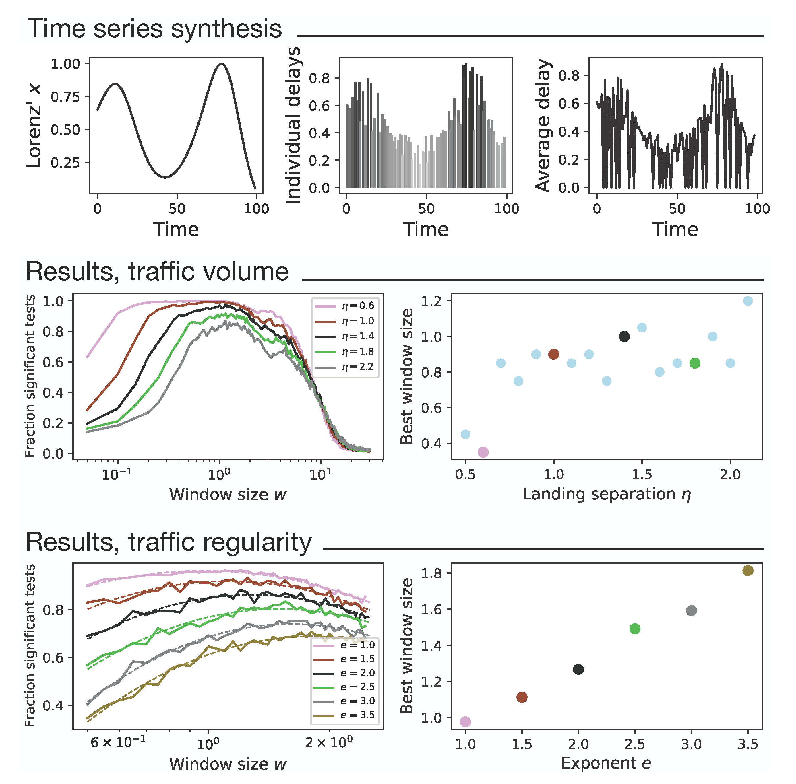
Once the two time series representing the overall evolution of delays have been created, it is necessary to reconstruct a set of landing events, as these are the only data available when analysing the real system. These events, for both the master and the dependent airports, are generated with a time separation between subsequent ones given by random numbers drawn from a uniform distribution . Thus, defines the expected separation between consecutive landings and is therefore inversely proportional to the amount of traffic. The delay assigned to each landing event is drawn from a second uniform distribution , where is the value of the variable x of the Lorenz model at time t. The result is then two sets of events representing synthetic delays, each one described by a time stamp and an observed landing delay. Finally, for a fixed value of w, we extract the average delay observed in non-overlapping windows of length w, both for the events of the master and the dependent airports. These averages are merged in two time series, which can then be analysed using the Granger causality test. Note that the detrend step is not necessary here, as the use of a chaotic system ensures the stationarity of the time series. An example of the generation of one average delay time series can be seen in Figure 1, top panels. From left to right, the three panels depict the generation of the Lorentz series representing the global evolution of delays, the generation of the landing events and the calculation of the average delays.
This model allows us to evaluate the behaviour of the Granger causality under well-controlled conditions. First of all, a causality is present between both time series by construction, as landing events in both airports are generated from time-shifted time series; it is thus possible to evaluate how sensitive the test actually is. Second, it is possible to fully control the parameters of the model and thus test the hypothesis that too small and too large values of w can result in an underestimation of the causality.
We proceed with the analysis of the model by varying the two main parameters: the average time between landing events and the window size w. For each combination of parameters, 1000 repetitions are generated, and the fraction of times that the p-value is significant is calculated.
The left middle panel of Figure 1 reports the proportion of significant tests for different window lengths w and for different event separation times . All plots follow a similar trend, where for very low values of the window length (between zero and one), most of the tests are not statistically significant, as not enough landing events are available to obtain meaningful average values. The fraction then increases until it reaches a maximum and finally decreases for large window lengths. This is different than that observed for small w, which is potentially due to the fact that too long a window results in the average of too much information, thus losing the high-frequency dynamics in both airports—or, in other words, that just the global average landing delay is obtained. The right middle panel of Figure 1 additionally reports a scatter plot of the optimal window size as a function of the separation time . In synthesis, the model confirms that an ideal (optimal) window size exists, for which the maximum number of causality relationships are detected; deviating from such an optimum results in an underestimation of the propagation.
We then change the simulation, specifically the synthesis of the landing events. The time separation between consecutive landings is now given by random numbers drawn from a distribution , e being an asymmetry exponent that stretches the positive tail of the distribution. In other words, while keeping the average constant, increasing this exponent results in clusters of landing events, with some of them happening after long periods of inactivity. Thus, this exponent is used to break the regularity of landing events and to simulate a more realistic burst distribution. We fix the average time between landing events and vary the window size w and the asymmetry exponent e; similar to before, we execute 1000 iterations for each pair of parameter values and record the proportion of times the p-value is significant.
The left bottom panel of Figure 1 depicts how the fraction of significant tests varies when considering different window sizes and asymmetry exponents. In order to compensate for the fluctuations due to the stochastic nature of the analysis, the dotted lines represent second order polynomial fits. The right bottom panel further depicts a scatter plot of the best window size as a function of the exponent e. A clear linear relation can be observed, where for larger asymmetry exponents, namely for less uniform separation times, the best window size grows; in other words, a larger window size is needed to detect causality relationships in order to cope with the periods of less activity.
In synthesis, results from the model confirm that the ideal window size to detect delay propagation is a function of the number of landing events; in other words, the higher the frequency with which we obtain information from the system, the higher the potential temporal resolution of the results. This optimum is a balance between two forces: the need for analysing large number of events to obtain a reliable average delay estimation, on one hand, and the risk of considering too long time windows, with the consequent smoothing of the fast part of the dynamics, on the other. Still, the estimation of such window length is made more complex by other factors, such as, for instance, the degree of regularity of landing events.
4. Analysis of Real Delay Propagation Patterns
When moving to the analysis of real delay data, the approach proposed here can be applied at three different levels. Firstly, there is a methodological point of view, i.e., one may simply be interested in optimising the analysis of delay propagation patterns and hence derive the best window size for detecting causality relationships. Secondly, such an optimal window size, along with the optimal lag as yielded by the Granger causality test, can be used to derive the time needed for delays to propagate between two airports. Finally, the last step is to move to a network level and see whether and how changing the window size modifies the resulting delay propagation topology. These three aspects will be tackled in this section.
4.1. Methodological Viewpoint: Best Time Scale for Detecting Delay Propagation
The identification of the best time scale for detecting delay propagation in real data is not dissimilar from what is presented in Figure 1; specifically, for a pair of target airports, one needs to reconstruct the corresponding delay time series for different values of w; to apply the Granger causality test, thus obtaining a p-value as a function of w and finally to select the w minimising such a p-value. Note that a smaller p-value implies a more statistically significant relationship, but also that such relationship manifests clearer in the data.
The top left panel of Figure 2 shows the window size w minimising the p-value, for those pairs of airports that display a statistically significant relationship (i.e., p-value , with a Bonferroni correction for multiple testing). No clear pattern can be discerned, with the optimal w varying from 30 min to up to two hour (see top right panel for a corresponding histogram). Specifically, no clear relationship seems to exist with the size of the airport (see middle right panel of Figure 2 representing a box plot of all ws for each airport and with airports sorted by decreasing number of operations and Figure A1, reporting a scatter plot of the optimal w as a function of the number of operations of airports).
Then, what are the elements that drive the size of such an optimal window? In order to answer this question, we extracted a set of time series describing the two most important aspects of the operations at an airport, i.e., the separation between landings and their delays—see the first column of Table A4. Each one of these sets of values has been synthesised using metrics such as the average or the standard deviation—second column of Table A4, and these features have further been combined for each pair of airports under analysis, using standard mathematical manipulations (e.g., the product or the maximum)—right columns of Table A4. The result is a set of 90 features per link. As a first approach, the linear correlation between each one of these features and the optimal w has been obtained, and the corresponding coefficient of determination has been calculated—see results in Table A4. Taken individually, none of them seem to substantially explain the best window size; the best result is given by the maximum of the median absolute deviation (MAD) of the landing times although the is only . We then exhaustively explored all combinations of four features and evaluated linear models based on them. The best four, yielding an of , are: the standard deviation of the landing separation for the receiving airport, the minimum Hurst exponent (HE) of the landing separation, the MAD of the landing times of the source airport, and the maximum of the MAD of the landing times. Scatter plots for these features and the corresponding linear fits are reported in the bottom panels of Figure 2. Finally, when combining all 90 features in a linear model, the resulting is .
What conclusions can be obtained from these results? From a general point of view, the landing and delay dynamics of the involved airports are partly responsible for defining the best window length w although a linear model can only explain of the variability. Additionally, it can be seen that such w depends mainly on the landing dynamics, with the delays themselves having a minor role—see Table A4. While selecting a few features is not enough to construct a model able to predict the best w, this latter seems to be related with the variability of the separation between consecutive landings, something that is in agreement with the results of Section 3.
In synthesis, obtaining the best window size w for a pair of airports is not a trivial process. Although it depends on the characteristics of the landing events, and specifically on the time between consecutive operations, the best w strongly changes between different pairs of airports, such that its value cannot be predicted at this stage. While disappointing, this is to be expected, as real operations (and data) are more complex than any synthetic model. Consequently, the only reliable alternative is testing several values of w and selecting the one yielding the minimal p-value.
4.2. Operational Viewpoint: Delay Propagation Time
Next, we tackle the problem of estimating the time it takes for delays to propagate within the network. This is achieved by considering the optimal window size w for each pair of airports, as estimated in the previous subsection, for then performing an exhaustive search to find the maximum lag yielding the best (lowest) p-value. Finally, the delay propagation time is obtained by multiplying these two values.
The left panel of Figure 3 reports the resulting delay propagation time for each pair of airports. As in the case of Figure 2, only results for those pairs of airports that have a statistically significant propagation are reported. Intuitively, one may hypothesise that such propagation time should be proportional to (or at least, be a function of) the distance between the two involved airports. As is evident in the scatter plot of the right panel of Figure 3, no simple pattern can be observed; a linear correlation analysis yields a coefficient of , with a p-value of .
We further estimate the time required for a delay to be propagated by an aircraft performing two consecutive flights, respectively, departing from airports a and c, as a function of the distance between the two airports. The geographical distance is transformed into time by considering a ground speed of 500 knots, plus one hour for departure and arrival procedures and turn-around operations. In other words, the objective is to obtain an estimation of the minimum time required between the two consecutive departures. The result is depicted by the dashed diagonal line in the right panel of Figure 3. It can be seen that most propagation times are well above the line, suggesting the presence of indirect propagation patterns—e.g., when the propagation between two airports a and c requires an intermediate airport b. This is consistent with the use of the Granger causality test, which is designed to detect these indirect patterns.
At the same time, a few pairs of airports have delays propagating between them in very short times, as low as 50 min—see Table A6. In other words, there are instances in which a delay takes less time to propagate than the duration of the shortest flight connecting the corresponding pair of airports. To illustrate this point, Figure 4 depicts a graphical representation of the five pairs of airports with the largest (red arrows), smallest (green arrows) and most asymmetrical (blue lines) propagation times—numerical data are reported in Table A5, Table A6 and Table A7. No clear trend can be identified. While most of the largest propagation times occur between distant airports, this also happens between Brussels and Hamburg and between Hamburg and Stuttgart. If delays between nearby airports are propagated by indirect connections, this does not explain the short time observed from Amsterdam and Hamburg or between Paris Orly and Stuttgart.
Following what was proposed in Ref. [12], the left panel of Figure 5 reports the distribution of the propagation time when airports are classified according to their size, i.e., in large and small ones—see also Figure A2 for full results. The former ones are those with a number of flights larger than the median of all considered airports; the latter ones are those with less flights. Four distributions of propagation times are then calculated corresponding to all possible combinations of airports at each end of a propagation link. As opposed to what was reported in Ref. [12], no significant differences can be observed. Additionally, the right panel of Figure 5 reports two distributions of the propagation times, respectively, corresponding to pairs of airports that are nearer or farther away than the median of all pairwise distances. While the propagation time is slightly larger for airports located farther away, the difference in medians is not statistically significant (Mood’s median test, p-value ).
We hypothesise that several factors may contribute to the complex relationship between the propagation time and airports’ characteristics. On one hand, it is clear that delays at neighbouring airports are influenced by shared weather patterns or even by interactions between their approach procedures. On the other hand, it is possible for information about delays to be transmitted before the corresponding flights reach their destination, as for instance when managed through ground delay programs. In short, it seems that the delay propagation time is driven by different and intermingling factors, including (but not exclusively) indirect connections and localised weather patterns.
4.3. Network Viewpoint: Propagation Network and Its Structure
The next logical step is to reconstruct the whole functional propagation network by varying the size of the window used to assess the Granger causality on the time series of pairs of airports. In Figure 6, blue lines report the evolution of six topological metrics as defined in Section 2.3 as a function of the window size used in the network reconstruction process. Note that this corresponds to the standard approach of using a single time scale for all possible propagation links. On the other hand, the dotted horizontal lines in the same figure report the network metrics when the optimal time scale is used for each airport pair.
Let us start by analysing the link density in the top left panel of Figure 6. It is apparent that using a fixed time window of 60 min, as common in the literature [15,16,17,18,19,20,21], leads to a significant information loss. In other words, and as seen in Figure 1, long windows imply a loss of information about the fast dynamics of delays and hence in an underestimation of the propagation. It is worth noting the magnitude of this effect: almost three-fourths of the causality links are lost for windows of 60 min compared to the use of optimal window lengths. At the same time, using very short time windows seems beneficial, with an increase in the link density. This is nevertheless misleading, as very short windows necessarily include more periods of inactivity—see the aqua line, right Y axis, representing the reliability, i.e., the fraction of airport pairs for which at least of the windows have one or more landing events. As previously discussed, these correspond to missing values, and it has been shown that too large a share of them results in an overestimation of the causality [33].
As to be expected, these changes in the link density, and hence in the number of detected links, have an impact on the values of all other topological metrics. Assortativity, transitivity and IC yield qualitatively similar values when comparing the results of using the optimal window size and a fixed 60 minimum one. The same is not true for the other two metrics, with the diameter and the efficiency being, respectively, under- and overestimated by using a fixed time window of 60 min. It is interesting to note that the former group of metrics are mostly local in nature, while the latter (i.e., those not correctly estimated) focuses on the macro-scale structure of the network. In other words, using a fixed (non-optimal) window size does not bias the structure created by pairs and triplets of airports, possibly those more strongly connected, but instead changes the overall structure of the propagation network.
To better understand how the centrality of the airports is modified by the use of different window sizes, Figure 7 reports the evolution of the airport ranking according to three centrality measures: in-degree, out-degree and betweenness centrality. Specifically, in each case, we consider the five airports that have the largest centrality when reconstructing the propagation network with the optimal window size and calculate the position in the ranking of these airports when considering a fixed window size. A simple look at Figure 7 shows that the window size has a profound effect on the centrality of airports, with these top five airports ending, in many cases, in the bottom half of the ranking. The sensitivity of the ranking to the window size is also noticeable, especially in the case of the betweenness. It is worth noting that this centrality metric strongly depends on the macro-scale structure of the network and that this result is therefore aligned with what is observed in Figure 6.
5. Resampling Validation
As a last point, we analyse another aspect that can influence the optimal window size for estimating the Granger causality. Several studies indicated that the sensitivity and stability of the test can be improved with higher temporal sampling rates [24,25]; this nevertheless can be due to two factors: the presence of new high-frequency information which is lost for low sampling rates or alternatively, the simple fact that longer time series (i.e., more data) make tests more statistically significant, even if no new information is included. Here, we approach this problem by leveraging the test suggested in Ref. [25] involving artificially resampling the analysed time series and comparing the evolution of the resulting p-values.
We start by considering the two original time series for a given pair of airports, reconstructed using the corresponding optimal window length. We then consider a resampling rate , and synthesise a new pair of time series by firstly downsampling the original data by a factor of and secondly upsampling them by the same factor. The result is a new set of time series whose length is preserved but in which high-frequency information is deleted. We finally compare the two p-values obtained with the original and resampled time series by calculating , where and represent the p-values obtained with, respectively, the resampled and original time series. Note that implies that the causality calculated with the resampled time series is stronger than that seen in the original case.
Figure 8 reports violin plots of the distribution of as a function of the resampling rate. In all cases, most are greater than zero—see also the aqua line, right Y axis, representing the percentage of links for which . In addition, the average of all distributions sits around five, thus indicating that the p-values for the original time series are significantly smaller than those for the resampled time series. In synthesis, one can conclude that the length of the optimal window is a function of the information the time series contains, specifically of its high-frequency part, and not directly of the time series length.
6. Discussion and Conclusions
In this paper, we have studied the effect of the temporal resolution used in the analysis of delay propagation in air transport, both in a synthetic model and in real operational data. While this is a problem well-known in the literature [24,25,26], air transport presents several idiosyncrasies, most notably the fact that events generating the time series (i.e., landings and their delays) are discrete. As shown in Section 3, the window size that maximises the sensitivity of a Granger causality test is a balance between several elements; in the simplest and noiseless case, it is between the need for detecting high-frequency dynamics through small windows and the need for windows long enough to contain a significant number of landing operations. Additional elements affecting the optimal window length include the presence of inactivity periods for which no events are available and the shape of the probability distribution of landing separation times, such that more heterogeneously spaced events require longer windows.
When applying these ideas to real data, three main conclusions can be drawn. First of all, due to the high complexity of real operations, the estimation of the best window size for a given airport pair can only be obtained numerically by systematically checking different window sizes and choosing the one minimising the test p-value. While these optima are related to some properties of the landing operations (see Figure 2), as previously discussed, such relationships are too weak to support the creation of an analytical solution. Secondly, the same approach can be used to infer the time required by delays to propagate between airports. Once again, results are loosely related to some airport characteristics, such as their distance and size, but no clear pattern can be discerned (see Figure 3). Thirdly, the use of a non-optimal window size has profound effects on the estimated structure of the delay propagation networks, with global features being more affected than micro-scale ones (see Figure 6).
It is worth noting that research works have hitherto used a fixed window length of one hour [15,16,17,18,19,20,21]. This prima facie made sense, as it is a natural way of dividing the day in equal parts; simplifies calculations, as windows of different days always start at the same time and is aligned with the way airport capacity is defined (i.e., operations per hour). We have nevertheless shown that the use of this fixed window substantially underestimates causality relationships and that the reconstructed network topology is thus misrepresented. This should be interpreted as a note of caution by the community, as previously published results may be partly incorrect. The present work is thus not only a theoretical exercise. Rather, it has direct implications on the analysis of real air transport delays.
Regarding the delay propagation times between pairs of airports reported in Figure 3, it is relevant to compare the results obtained here with those of Ref. [12]. Specifically, those authors reported a correlation between the distance between two airports and the corresponding propagation timescale, and the latter was also modified by the role of the airport in the network (e.g., hub vs. peripheral airport), albeit to a lesser degree. Similar trends can be observed in our results, albeit they never are statistically significant (see Figure 3 and Figure 5). Several causes can explain such a discrepancy. First of all, the detection of the delay propagation patterns and the estimation of their time scale is performed in Ref. [12] by using lagged linear correlations as opposed to the Granger causality considered here. Significant differences ought to be expected, especially taking into account that the Granger test is designed to detect indirect propagation patterns, i.e., when delays propagate between two airports through an intervening one. Secondly, Ref. [12] is based on the use of windows of a fixed size of 30 min; even though the analysis is based on a different technique to detect the delay propagation, the use of a fixed window length seems sub-optimal in light of what is presented here. Thirdly, the possibility that differences between the US and European systems, e.g., in the management of delays [61,62], could be the basis of such discrepancies cannot be ruled out.
Future works will have to be targeted at confirming and extending the results obtained here. Firstly, given the variability observed when changing the temporal scale of the time series reconstruction, it stands to reason to expect even more heterogeneous results when links are obtained with different metrics, e.g., correlation or non-linear causality ones. Specifically, non-linear causality metrics, such as non-linear versions of the Granger causality [42,63,64] or the Transfer Entropy [65], usually require longer time series to obtain reliable results. As a consequence, correctly estimating the optimal time scale may become even more critical. Secondly, similar analyses could be performed when considering alternative ways of reconstructing delay time series, e.g., by analysing each airline independently [15], thus effectively moving from a single- to a multi-layer representation [66], or by estimating the departure (as opposed to arrival) delays. Thirdly, it would be interesting to check whether similar results are also obtained in other large air transport systems, e.g., the US or Chinese ones. It would also simplify future studies to have an explicit a priori estimation of the optimal window length, for instance obtained through a machine learning model trained over a large set of airports and their operations.
As a final note of caution, it is worth recalling that functional networks are a powerful tool to describe delay propagation patterns in air transport, as customarily conducted in other scientific fields [44,45,46,47,48,49]. At the same time, this kind of analysis provides little information about the factors and reasons behind them. In other words, they allow to describe, but not to explain the dynamics of delay propagation. While it is in principle possible to combine functional network representations with other operational data, and hence understand if and how much the latter affect the former, this has yet to be accomplished and represents an open field of research.
Author Contributions
Conceptualization, M.Z.; formal analysis, L.P.; data curation, L.P.; writing—original draft preparation, L.P. and M.Z.; writing—review and editing, L.P. and M.Z. All authors have read and agreed to the published version of the manuscript.
Funding
This project has received funding from the European Research Council (ERC) under the European Union’s Horizon 2020 research and innovation programme (grant agreement No 851255). Authors acknowledge the Spanish State Research Agency through Grant MDM-2017-0711 funded by MCIN/AEI/10.13039/501100011033.
Institutional Review Board Statement
Not applicable.
Informed Consent Statement
Not applicable.
Data Availability Statement
The data that support the findings of this study are openly available at https://www.eurocontrol.int/dashboard/rnd-data-archive (accessed on 11 February 2022).
Conflicts of Interest
The authors declare no conflict of interest.
Appendix A

Table A1.
Information on the 50 airports considered in this study, including their 4-letter ICAO code, number of landing flights and percentage of flights delayed more than 10 and 30 min.
Table A1.
Information on the 50 airports considered in this study, including their 4-letter ICAO code, number of landing flights and percentage of flights delayed more than 10 and 30 min.
| Rank | Name | ICAO | # Flights | % Delayed > 10 min. | % Delayed > 30 min. |
|---|---|---|---|---|---|
| 1 | Frankfurt Airport | EDDF | 23,061 | 30.65% | 5.06% |
| 2 | Amsterdam Airport Schiphol | EHAM | 22,350 | 52.77% | 11.55% |
| 3 | Paris Charles de Gaulle Airport | LFPG | 22,275 | 33.76% | 5.39% |
| 4 | London Heathrow | EGLL | 19,407 | 68.39% | 20.39% |
| 5 | Munich Airport | EDDM | 18,588 | 25.22% | 2.75% |
| 6 | Adolfo Suárez Madrid-Barajas Airport | LEMD | 18,345 | 38.50% | 7.44% |
| 7 | Josep Tarradellas Barcelona-El Prat Airport | LEBL | 15,817 | 44.39% | 10.14% |
| 8 | Rome-Fiumicino International Airport | LIRF | 13,930 | 14.45% | 2.84% |
| 9 | Milan Malpensa Airport | LIMC | 13,383 | 12.67% | 2.84% |
| 10 | London Gatwick Airport | EGKK | 12,985 | 61.29% | 18.78% |
| 11 | Palma de Mallorca Airport | LEPA | 12,616 | 32.13% | 10.03% |
| 12 | Vienna International Airport | LOWW | 12,482 | 42.16% | 7.34% |
| 13 | Copenhagen Kastrup Airport | EKCH | 11,811 | 18.72% | 2.24% |
| 14 | Zürich Airport | LSZH | 11,426 | 41.24% | 5.56% |
| 15 | Oslo Airport | ENGM | 11,203 | 12.79% | 1.11% |
| 16 | Athens Intl Eleftherios Venizelos | LGAV | 10,808 | 25.54% | 3.22% |
| 17 | Dublin Airport | EIDW | 10,731 | 26.94% | 4.63% |
| 18 | Stockholm Arlanda Airport | ESSA | 10,585 | 22.57% | 2.51% |
| 19 | Brussels Airport | EBBR | 10,313 | 40.79% | 6.73% |
| 20 | Düsseldorf Airport | EDDL | 10,178 | 33.52% | 4.87% |
| 21 | Humberto Delgado Airport | LPPT | 9852 | 45.98% | 8.10% |
| 22 | Manchester Airport | EGCC | 9635 | 39.81% | 6.58% |
| 23 | Paris Orly Airport | LFPO | 9283 | 30.09% | 4.73% |
| 24 | London Stansted Airport | EGSS | 8634 | 41.52% | 6.24% |
| 25 | Berlin Tegel “Otto Lilienthal” Airport | EDDT | 8545 | 27.55% | 3.25% |
| 26 | Warsaw Chopin Airport | EPWA | 8434 | 10.91% | 1.67% |
| 27 | Václav Havel Airport Prague | LKPR | 7263 | 24.03% | 3.33% |
| 28 | Geneva Airport | LSGG | 7108 | 25.63% | 4.47% |
| 29 | Nice Côte d’Azur Airport | LFMN | 6703 | 20.50% | 3.43% |
| 30 | Málaga-Costa del Sol Airport | LEMG | 6660 | 35.47% | 4.76% |
| 31 | Hamburg Airport | EDDH | 6531 | 21.45% | 2.56% |
| 32 | Cologne Bonn Airport | EDDK | 6423 | 26.48% | 3.30% |
| 33 | London Luton Airport | EGGW | 6103 | 46.53% | 8.65% |
| 34 | Stuttgart Airport | EDDS | 6066 | 28.70% | 3.07% |
| 35 | Edinburgh Airport | EGPH | 5843 | 21.80% | 2.57% |
| 36 | Boryspil International Airport | UKBB | 5620 | 22.94% | 2.74% |
| 37 | Budapest Ferenc Liszt International Airport | LHBP | 5452 | 17.59% | 2.27% |
| 38 | Bucharest Henri Coandă International Airport | LROP | 5390 | 13.36% | 1.78% |
| 39 | Lyon-Saint Exupéry Airport | LFLL | 5127 | 26.41% | 3.49% |
| 40 | Alicante-Elche Miguel Hernández Airport | LEAL | 4946 | 34.17% | 5.14% |
| 41 | Birmingham Airport | EGBB | 4891 | 20.40% | 2.25% |
| 42 | Venice Marco Polo Airport | LIPZ | 4720 | 27.58% | 5.76% |
| 43 | Francisco Sá Carneiro Airport | LPPR | 4443 | 38.06% | 10.44% |
| 44 | Orio al Serio International Airport | LIME | 4417 | 16.32% | 2.04% |
| 45 | Marseille Provence Airport | LFML | 4329 | 23.56% | 2.73% |
| 46 | Toulouse-Blagnac Airport | LFBO | 4159 | 17.62% | 1.90% |
| 47 | Naples International Airport | LIRN | 4041 | 27.86% | 3.07% |
| 48 | Glasgow Airport | EGPF | 3732 | 28.27% | 3.99% |
| 49 | Catania-Fontanarossa Airport | LICC | 3660 | 14.64% | 1.53% |
| 50 | Bologna Guglielmo Marconi Airport | LIPE | 3519 | 25.09% | 2.90% |
Table A2.
Formal definition of the network topological metrics considered in this study.
| Metric | Definition | Range |
|---|---|---|
| Link density | , | |
| L being the total number of active links in the network and N the number of nodes. | ||
| Diameter | , | |
| being the distance between nodes i and j | ||
| Transitivity | ||
| being the number of closed triangles , and the number of connected triplets . | ||
| Assortativity | , | |
| j and k being the degrees of nodes at each end of a link; the distribution of the remaining degree, i.e., of the degree without the link under study; the variance of the distribution ; and the joint probability distribution of the remaining degrees of the two vertices at either end of a randomly chosen link. | ||
| Efficiency | , | |
| being the distance between the nodes i and j. | ||
| Information Content | See [55] |
Table A3.
Formal definition of the centrality metrics considered in this study. Note that these metrics are calculated for a single node (here denoted as w), as opposed to the whole network; nodes can then be ranked in importance accordingly.
Table A3.
Formal definition of the centrality metrics considered in this study. Note that these metrics are calculated for a single node (here denoted as w), as opposed to the whole network; nodes can then be ranked in importance accordingly.
| Centrality Metric | Definition |
|---|---|
| Out-degree centrality | , |
| where is equal to one if a link exists between nodes w and j, and zero otherwise. | |
| In-degree centrality | , |
| where is equal to one if a link exists between nodes j and w, and zero otherwise. | |
| Betweenness centrality | , |
| where V is the set of nodes, the number of shortest paths between s and t, and the number of shortest paths between s and t that includes w. |
Figure A1.
Scatter plot of the length of the optimal window for each pair of airports as a function of the number of operations recorded in the data set for the source (X axis) and destination (Y axis) airports.
Figure A1.
Scatter plot of the length of the optimal window for each pair of airports as a function of the number of operations recorded in the data set for the source (X axis) and destination (Y axis) airports.

Table A4.
Coefficients of determination obtained by fitting linear models to recover the best window size for each pair of airports, using the corresponding features listed in the left columns; a: source airport of the causality (i.e., the cause); b: destination airport of the causality (i.e., the consequence).
| Input Time | Metric | ||||||
|---|---|---|---|---|---|---|---|
| Series | a | b | Max | Min | |||
| Landing times | MAD | ||||||
| Hurst exponent | |||||||
| Landing separation | Mean | ||||||
| Standard deviation | |||||||
| Linear correlation | |||||||
| MAD | |||||||
| Delays | Mean | ||||||
| Standard deviation | |||||||
| Linear correlation | |||||||
| MAD | |||||||
| Hurst exponent | |||||||
| consecutive delays | Mean | ||||||
| Standard deviation | |||||||
| Linear correlation | |||||||
| MAD | |||||||
Table A5.
List of the ten pairs of airports with the longest propagation time (in hours); a: source airport of the causality (i.e., the cause); b: destination airport of the causality (i.e., the consequence).
Table A5.
List of the ten pairs of airports with the longest propagation time (in hours); a: source airport of the causality (i.e., the cause); b: destination airport of the causality (i.e., the consequence).
| Airport a | Airport b | Distance (NM) | Prop. Time |
|---|---|---|---|
| EBBR | EDDH | 482 | 8.0 |
| LIME | LEMG | 1549 | 8.0 |
| EDDH | EDDS | 552 | 7.5 |
| EDDT | LPPR | 2077 | 7.3 |
| LEBL | LHBP | 1523 | 7.1 |
| EBBR | EGBB | 463 | 7.1 |
| LIMC | LOWW | 657 | 7.1 |
| LIMC | LKPR | 646 | 7.1 |
| LIME | LOWW | 588 | 7.1 |
| EGBB | EBBR | 463 | 7.1 |
Table A6.
List of the ten pairs of airports with the shortest propagation time (in hours); a: source airport of the causality (i.e., the cause); b: destination airport of the causality (i.e., the consequence).
Table A6.
List of the ten pairs of airports with the shortest propagation time (in hours); a: source airport of the causality (i.e., the cause); b: destination airport of the causality (i.e., the consequence).
| Airport a | Airport b | Distance (NM) | Prop. Time |
|---|---|---|---|
| LFPO | EDDS | 502 | 0.8 |
| UKBB | LGAV | 1485 | 1.0 |
| EDDS | LFPO | 502 | 1.2 |
| EHAM | EDDH | 379 | 1.2 |
| LIML | ENGM | 1645 | 1.4 |
| LGAV | UKBB | 1485 | 1.8 |
| EDDS | EDDH | 552 | 1.8 |
| LFML | ENGM | 1906 | 2.0 |
| ENGM | EDDS | 1286 | 2.0 |
| LSZH | EPWA | 1031 | 2.2 |
Table A7.
List of the ten pairs of airports with the most asymmetrical propagation time, defined as the difference between the forward (reported in the fourth column) and backward time (fifth column); a: source airport of the causality (i.e., the cause); b: destination airport of the causality (i.e., the consequence). Propagation times in hours.
| Airport a | Airport b | Distance (NM) | Prop. Time | Prop. Time |
|---|---|---|---|---|
| EDDH | EDDS | 552 | 7.5 | 1.8 |
| LIME | LEMG | 1549 | 8.0 | 3.7 |
| EBBR | EDDH | 482 | 8.0 | 4.0 |
| LICC | LSGG | 1223 | 6.5 | 4.2 |
| EKCH | ESSA | 546 | 7.0 | 5.2 |
| LIMC | EDDS | 342 | 6.8 | 5.0 |
| LGAV | LPPR | 2803 | 7.0 | 5.7 |
| LIMC | EHAM | 795 | 7.0 | 5.8 |
| LIMC | LOWW | 657 | 7.1 | 6.0 |
| LIME | LOWW | 588 | 7.1 | 6.0 |
Figure A2.
Probability distributions of delay propagation times. Violin plots report the distribution of the delay propagation times in hours for all 50 considered airports for outgoing (i.e., delays propagated by an airport, top panels) and incoming (i.e., delays received by an airport, bottom panels) links.

References
- Rantanen, E.M.; Wickens, C.D. Conflict resolution maneuvers in air traffic control: Investigation of operational data. Int. J. Aviat. Psychol. 2012, 22, 266–281. [Google Scholar] [CrossRef]
- Shang-Wen, Y.; Ming-Hua, H. Estimation of air traffic longitudinal conflict probability based on the reaction time of controllers. Saf. Sci. 2010, 48, 926–930. [Google Scholar] [CrossRef]
- Delgado, L.; Martin, J.; Blanch, A.; Cristóbal, S. Hub operations delay recovery based on cost optimisation-Dynamic cost indexing and waiting for passengers strategies. In Sixth SESAR Innovation Days; SESAR: Brussels, Belgium, 2016. [Google Scholar]
- Montlaur, A.; Delgado, L. Flight and passenger delay assignment optimization strategies. Transp. Res. Part C Emerg. Technol. 2017, 81, 99–117. [Google Scholar] [CrossRef] [Green Version]
- Pyrgiotis, N.; Malone, K.M.; Odoni, A. Modelling delay propagation within an airport network. Transp. Res. Part C Emerg. Technol. 2013, 27, 60–75. [Google Scholar] [CrossRef]
- Beatty, R.; Hsu, R.; Berry, L.; Rome, J. Preliminary evaluation of flight delay propagation through an airline schedule. Air Traffic Control. Q. 1999, 7, 259–270. [Google Scholar] [CrossRef]
- Liu, Y.J.; Cao, W.D.; Ma, S. Estimation of arrival flight delay and delay propagation in a busy hub-airport. In Proceedings of the IEEE 2008 Fourth International Conference on Natural Computation, Jinan, China, 18–20 October 2008; Volume 4, pp. 500–505. [Google Scholar]
- AhmadBeygi, S.; Cohn, A.; Guan, Y.; Belobaba, P. Analysis of the potential for delay propagation in passenger airline networks. J. Air Transp. Manag. 2008, 14, 221–236. [Google Scholar] [CrossRef] [Green Version]
- Fleurquin, P.; Ramasco, J.J.; Eguiluz, V.M. Systemic delay propagation in the US airport network. Sci. Rep. 2013, 3, 1159. [Google Scholar] [CrossRef] [Green Version]
- Baspinar, B.; Koyuncu, E. A data-driven air transportation delay propagation model using epidemic process models. Int. J. Aerosp. Eng. 2016, 2016, 4836260. [Google Scholar] [CrossRef]
- Zhang, H.; Wu, W.; Zhang, S.; Witlox, F. Simulation analysis on flight delay propagation under different network configurations. IEEE Access 2020, 8, 103236–103244. [Google Scholar] [CrossRef]
- Wang, Y.; Li, M.Z.; Gopalakrishnan, K.; Liu, T. Timescales of delay propagation in airport networks. Transp. Res. Part E Logist. Transp. Rev. 2022, 161, 102687. [Google Scholar] [CrossRef]
- Granger, C.W. Investigating causal relations by econometric models and cross-spectral methods. Econom. J. Econom. Soc. 1969, 37, 424–438. [Google Scholar] [CrossRef]
- Granger, C.W. Causality, cointegration, and control. J. Econ. Dyn. Control. 1988, 12, 551–559. [Google Scholar] [CrossRef]
- Zanin, M. Can we neglect the multi-layer structure of functional networks? Phys. A Stat. Mech. Its Appl. 2015, 430, 184–192. [Google Scholar] [CrossRef] [Green Version]
- Zanin, M.; Belkoura, S.; Zhu, Y. Network analysis of chinese air transport delay propagation. Chin. J. Aeronaut. 2017, 30, 491–499. [Google Scholar] [CrossRef]
- Du, W.B.; Zhang, M.Y.; Zhang, Y.; Cao, X.B.; Zhang, J. Delay causality network in air transport systems. Transp. Res. Part E Logist. Transp. Rev. 2018, 118, 466–476. [Google Scholar] [CrossRef]
- Mazzarisi, P.; Zaoli, S.; Lillo, F.; Delgado, L.; Gurtner, G. New centrality and causality metrics assessing air traffic network interactions. J. Air Transp. Manag. 2020, 85, 101801. [Google Scholar] [CrossRef] [Green Version]
- Pastorino, L.; Zanin, M. Air delay propagation patterns in Europe from 2015 to 2018: An information processing perspective. J. Phys. Complex. 2021, 3, 015001. [Google Scholar] [CrossRef]
- Guo, Z.; Hao, M.; Yu, B.; Yao, B. Detecting delay propagation in regional air transport systems using convergent cross mapping and complex network theory. Transp. Res. Part E Logist. Transp. Rev. 2022, 157, 102585. [Google Scholar] [CrossRef]
- Jia, Z.; Cai, X.; Hu, Y.; Ji, J.; Jiao, Z. Delay propagation network in air transport systems based on refined nonlinear Granger causality. Transp. B Transp. Dyn. 2022, 10, 586–598. [Google Scholar] [CrossRef]
- Costa, L.d.F.; Rodrigues, F.A.; Travieso, G.; Villas Boas, P.R. Characterization of complex networks: A survey of measurements. Adv. Phys. 2007, 56, 167–242. [Google Scholar] [CrossRef]
- Zanin, M. Simplifying functional network representation and interpretation through causality clustering. Sci. Rep. 2021, 11, 15378. [Google Scholar] [CrossRef] [PubMed]
- Gong, M.; Zhang, K.; Schoelkopf, B.; Tao, D.; Geiger, P. Discovering temporal causal relations from subsampled data. In Proceedings of the International Conference on Machine Learning, PMLR, Lille, France, 6–11 July 2015; pp. 1898–1906. [Google Scholar]
- Lin, F.H.; Ahveninen, J.; Raij, T.; Witzel, T.; Chu, Y.H.; Jääskeläinen, I.P.; Tsai, K.W.K.; Kuo, W.J.; Belliveau, J.W. Increasing fMRI sampling rate improves Granger causality estimates. PLoS ONE 2014, 9, e100319. [Google Scholar] [CrossRef] [PubMed] [Green Version]
- Zhou, D.; Zhang, Y.; Xiao, Y.; Cai, D. Reliability of the Granger causality inference. New J. Phys. 2014, 16, 043016. [Google Scholar] [CrossRef] [Green Version]
- Renault, E.; Sekkat, K.; Szafarz, A. Testing for spurious causality in exchange rates. J. Empir. Financ. 1998, 5, 47–66. [Google Scholar] [CrossRef]
- McCrorie, J.R.; Chambers, M.J. Granger causality and the sampling of economic processes. J. Econom. 2006, 132, 311–336. [Google Scholar] [CrossRef] [Green Version]
- Solo, V. On causality I: Sampling and noise. In Proceedings of the IEEE 2007 46th IEEE Conference on Decision and Control, New Orleans, LA, USA, 12–14 December 2007; pp. 3634–3639. [Google Scholar]
- Smirnov, D.; Bezruchko, B. Spurious causalities due to low temporal resolution: Towards detection of bidirectional coupling from time series. EPL (Europhys. Lett.) 2012, 100, 10005. [Google Scholar] [CrossRef] [Green Version]
- Anderson, B.D.; Deistler, M.; Dufour, J.M. On the Sensitivity of Granger causality to Errors-In-Variables, Linear Transformations and Subsampling. J. Time Ser. Anal. 2019, 40, 102–123. [Google Scholar] [CrossRef] [Green Version]
- Elsegai, H. Granger-causality inference in the presence of gaps: An equidistant missing-data problem for non-synchronous recorded time series data. Phys. A Stat. Mech. Its Appl. 2019, 523, 839–851. [Google Scholar] [CrossRef]
- Zanin, M. Assessing Granger causality on irregular missing and extreme data. IEEE Access 2021, 9, 75362–75374. [Google Scholar] [CrossRef]
- Bessler, D.A.; Kling, J.L. A note on tests of Granger causality. Appl. Econ. 1984, 16, 335–342. [Google Scholar] [CrossRef]
- Joerding, W. Economic growth and defense spending: Granger causality. J. Dev. Econ. 1986, 21, 35–40. [Google Scholar] [CrossRef]
- Chiou-Wei, S.Z.; Chen, C.F.; Zhu, Z. Economic growth and energy consumption revisited—Evidence from linear and nonlinear Granger causality. Energy Econ. 2008, 30, 3063–3076. [Google Scholar] [CrossRef]
- Yuan, T.; Qin, S. Root cause diagnosis of plant-wide oscillations using Granger causality. J. Process. Control. 2014, 24, 450–459. [Google Scholar] [CrossRef]
- Seth, A.K.; Barrett, A.B.; Barnett, L. Granger causality Analysis in Neuroscience and Neuroimaging. J. Neurosci. 2015, 35, 3293–3297. [Google Scholar] [CrossRef] [PubMed]
- Stokes, P.A.; Purdon, P.L. A study of problems encountered in Granger causality analysis from a neuroscience perspective. Proc. Natl. Acad. Sci. USA 2017, 114, E7063–E7072. [Google Scholar] [CrossRef] [Green Version]
- Porta, A.; Faes, L. Wiener–Granger causality in Network Physiology with Applications to Cardiovascular Control and Neuroscience. Proc. IEEE 2016, 104, 282–309. [Google Scholar] [CrossRef]
- Dhamala, M.; Rangarajan, G.; Ding, M. Estimating Granger causality from Fourier and wavelet transforms of time series data. Phys. Rev. Lett. 2008, 100, 018701. [Google Scholar] [CrossRef] [Green Version]
- Marinazzo, D.; Pellicoro, M.; Stramaglia, S. Kernel method for nonlinear Granger causality. Phys. Rev. Lett. 2008, 100, 144103. [Google Scholar] [CrossRef] [Green Version]
- Bueso, D.; Piles, M.; Camps-Valls, G. Explicit Granger causality in kernel Hilbert spaces. Phys. Rev. E 2020, 102, 062201. [Google Scholar] [CrossRef]
- Bullmore, E.; Sporns, O. Complex brain networks: Graph theoretical analysis of structural and functional systems. Nat. Rev. Neurosci. 2009, 10, 186–198. [Google Scholar] [CrossRef]
- Park, H.J.; Friston, K. Structural and functional brain networks: From connections to cognition. Science 2013, 342, 1238411. [Google Scholar] [CrossRef] [Green Version]
- Sporns, O. Graph theory methods: Applications in brain networks. Dialogues Clin. Neurosci. 2022, 20, 111–121. [Google Scholar] [CrossRef] [PubMed]
- Donges, J.F.; Zou, Y.; Marwan, N.; Kurths, J. Complex networks in climate dynamics. Eur. Phys. J. Spec. Top. 2009, 174, 157–179. [Google Scholar] [CrossRef] [Green Version]
- Donges, J.F.; Zou, Y.; Marwan, N.; Kurths, J. The backbone of the climate network. EPL (Europhys. Lett.) 2009, 87, 48007. [Google Scholar] [CrossRef] [Green Version]
- Ludescher, J.; Martin, M.; Boers, N.; Bunde, A.; Ciemer, C.; Fan, J.; Havlin, S.; Kretschmer, M.; Kurths, J.; Runge, J.; et al. Network-based forecasting of climate phenomena. Proc. Natl. Acad. Sci. USA 2021, 118, e1922872118. [Google Scholar] [CrossRef]
- Albert, R.; Barabási, A.L. Statistical mechanics of complex networks. Rev. Mod. Phys. 2002, 74, 47. [Google Scholar] [CrossRef] [Green Version]
- Boccaletti, S.; Latora, V.; Moreno, Y.; Chavez, M.; Hwang, D.U. Complex networks: Structure and dynamics. Phys. Rep. 2006, 424, 175–308. [Google Scholar] [CrossRef]
- Newman, M.E. Assortative mixing in networks. Phys. Rev. Lett. 2002, 89, 208701. [Google Scholar] [CrossRef] [Green Version]
- Latora, V.; Marchiori, M. Efficient behavior of small-world networks. Phys. Rev. Lett. 2001, 87, 198701. [Google Scholar] [CrossRef] [Green Version]
- Crucitti, P.; Latora, V.; Marchiori, M.; Rapisarda, A. Efficiency of scale-free networks: Error and attack tolerance. Phys. A Stat. Mech. Its Appl. 2003, 320, 622–642. [Google Scholar] [CrossRef]
- Zanin, M.; Sousa, P.A.; Menasalvas, E. Information content: Assessing meso-scale structures in complex networks. EPL (Europhys. Lett.) 2014, 106, 30001. [Google Scholar] [CrossRef] [Green Version]
- Bonacich, P. Power and centrality: A family of measures. Am. J. Sociol. 1987, 92, 1170–1182. [Google Scholar] [CrossRef]
- Zanin, M.; Sun, X.; Wandelt, S. Studying the topology of transportation systems through complex networks: Handle with care. J. Adv. Transp. 2018, 2018, 3156137. [Google Scholar] [CrossRef] [Green Version]
- Tabor, M.; Weiss, J. Analytic structure of the Lorenz system. Phys. Rev. A 1981, 24, 2157. [Google Scholar] [CrossRef]
- Brock, W.A.; Malliaris, A.G. Differential Equations, Stability and Chaos in Dynamic Economics; World Scientific: Amsterdam, The Netherlands, 1989. [Google Scholar]
- Coffey, D.S. Self-organization, complexity and chaos: The new biology for medicine. Nat. Med. 1998, 4, 882–885. [Google Scholar] [CrossRef]
- Campanelli, B.; Fleurquin, P.; Arranz, A.; Etxebarria, I.; Ciruelos, C.; Eguíluz, V.M.; Ramasco, J.J. Comparing the modeling of delay propagation in the US and European air traffic networks. J. Air Transp. Manag. 2016, 56, 12–18. [Google Scholar] [CrossRef]
- Cook, A.; Belkoura, S.; Zanin, M. ATM performance measurement in Europe, the US and China. Chin. J. Aeronaut. 2017, 30, 479–490. [Google Scholar] [CrossRef]
- Sun, X. Assessing nonlinear Granger causality from multivariate time series. In Proceedings of the Joint European Conference on Machine Learning and Knowledge Discovery in Databases; Springer: Berlin/Heidelberg, Germany, 2008; pp. 440–455. [Google Scholar]
- Song, X.; Taamouti, A. Measuring nonlinear granger causality in mean. J. Bus. Econ. Stat. 2018, 36, 321–333. [Google Scholar] [CrossRef] [Green Version]
- Staniek, M.; Lehnertz, K. Symbolic transfer entropy. Phys. Rev. Lett. 2008, 100, 158101. [Google Scholar] [CrossRef]
- Boccaletti, S.; Bianconi, G.; Criado, R.; Del Genio, C.I.; Gómez-Gardenes, J.; Romance, M.; Sendina-Nadal, I.; Wang, Z.; Zanin, M. The structure and dynamics of multilayer networks. Phys. Rep. 2014, 544, 1–122. [Google Scholar] [CrossRef]
Figure 1.
Analysis of the synthetic model—see Section 3 for details. (Top panels) Example of the synthesis of one time series, with the calculation of the global delay trend using a Lorenz system (top left panel); synthesis of individual landing events (top central panel); and reconstruction of the evolution of the average delay (top right panel); (Middle panels) Analysis of the Granger causality test as a function of the traffic volume: evolution of the fraction of significant tests as a function of the window size w and of the event separation time ; (left middle panel); and size of the best window size, i.e., the one maximising the fraction of significant tests for different values of (right middle panel); (Bottom panels) Analysis of the Granger causality test as a function of the traffic regularity: evolution of the fraction of significant tests as a function of w and of the asymmetry exponent e (left bottom panel); and value of w maximising that fraction as a function of e, as obtained from the quadratic fits (right bottom panel). In the middle and bottom panels, coloured points in the right panels correspond to the line of the same colour in the left ones.

Figure 2.
Best time scale for detecting real delay propagation patterns. (Top left) window length minimising the p-value of the Granger causality test for each pair of source–destination airports; note that results are only reported for those pairs for which the test is statistically significant and that airports are sorted in decreasing number of operations (see Table A1); (Top right) histogram of the best window lengths w; (Middle right) box plot depicting the distribution of the best window lengths for each airport, considering the links it causes, with airports sorted by decreasing number of operations; boxes indicate the interquartile range (Q3–Q1) and blue horizontal lines the median of the distribution; (Bottom) scatter plots of the four features that best predict the length of the optimal window as a function of the latter for each statistically significant causality link; the black lines represent the best linear fit. L. sep.: landing separation; L. time: landing time. See main text and Table A4 for details on the metrics.

Figure 3.
Delay propagation time. The left panel reports the delay propagation time in hours between each pair of airports. Only pairs with a statistically significant propagation are reported, and airports are sorted in decreasing number of operations (see Table A1). The right panel represents a scatter plot of the propagation time in hours as a function of the distance between each pair of airports. The diagonal dotted line approximates the flight time as a function of the distance.

Figure 4.
Graphical representation of the most extreme delay propagation times. Red and green arrows indicate the five pairs of airports with, respectively, the largest and smallest propagation times; blue lines indicate those pairs with the most asymmetrical ones. See Table A5, Table A6 and Table A7 for numerical values.

Figure 5.
Violin plots reporting the distributions of propagation times as a function of the size of the airports at each end of the link (left panel) and of the distance between them (right panel). L: large; S: small.
Figure 5.
Violin plots reporting the distributions of propagation times as a function of the size of the airports at each end of the link (left panel) and of the distance between them (right panel). L: large; S: small.

Figure 6.
Evolution of the six topological metrics described in Section 2.3 (blue lines, left Y axes), as a function of the size of the window used for calculating the Granger causality. Aqua lines (right Y axes) depict the reliability of each value, i.e., the fraction of pairs of airports having operations in at least of the windows used to calculate the causality. The horizontal dotted lines indicate the values of the metrics when the optimal window size is used for each link.

Figure 7.
Evolution of the centrality ranking as a function of the window size used to calculate the Granger causality. From left to right, the three panels depict the evolution of the ranking according to the out-degree, in-degree and betweenness centrality. In each case, the five reported airports are those with the maximal centrality in the networks reconstructed with optimal window sizes.

Figure 8.
Probability distribution of , i.e., the difference between the p-values obtained with the original and the resampled time series. Each violin plot corresponds to a different resampling, and its values to all pairs of airports with a statistically significant causality (according to the original time series). The water green line (right Y axis) shows the percentage of pairs for which the resampled time series yield a smaller p-value (that is, a more statistically significant relationship) than the one obtained with the original series.

Disclaimer/Publisher’s Note: The statements, opinions and data contained in all publications are solely those of the individual author(s) and contributor(s) and not of MDPI and/or the editor(s). MDPI and/or the editor(s) disclaim responsibility for any injury to people or property resulting from any ideas, methods, instructions or products referred to in the content. |
© 2023 by the authors. Licensee MDPI, Basel, Switzerland. This article is an open access article distributed under the terms and conditions of the Creative Commons Attribution (CC BY) license (https://creativecommons.org/licenses/by/4.0/).
Share and Cite
MDPI and ACS Style
Pastorino, L.; Zanin, M. Local and Network-Wide Time Scales of Delay Propagation in Air Transport: A Granger Causality Approach. Aerospace 2023, 10, 36. https://doi.org/10.3390/aerospace10010036
AMA Style
Pastorino L, Zanin M. Local and Network-Wide Time Scales of Delay Propagation in Air Transport: A Granger Causality Approach. Aerospace. 2023; 10(1):36. https://doi.org/10.3390/aerospace10010036
Chicago/Turabian StylePastorino, Luisina, and Massimiliano Zanin. 2023. "Local and Network-Wide Time Scales of Delay Propagation in Air Transport: A Granger Causality Approach" Aerospace 10, no. 1: 36. https://doi.org/10.3390/aerospace10010036
Note that from the first issue of 2016, this journal uses article numbers instead of page numbers. See further details here.