
Modeling and Design Optimization of an Electric Environmental Control System for Commercial Passenger Aircraft

ISAE-SUPAERO, Université de Toulouse, 31055 Toulouse, France
*
Author to whom correspondence should be addressed.
Aerospace 2023, 10(3), 260; https://doi.org/10.3390/aerospace10030260
Submission received: 16 January 2023
/
Revised: 7 February 2023
/
Accepted: 6 March 2023
/
Published: 8 March 2023
(This article belongs to the Section Aeronautics)
Abstract
:The aircraft environmental control system (ECS) is the second-highest fuel consumer system, behind the propulsion system. To reduce fuel consumption, one research direction intends to replace conventional aircraft with more electric aircraft. Thus, new electric architectures have to be designed for each system, such as for the ECS. In this paper, an electric ECS is modeled and then sized and optimized for different sizing scenarios with the aim of minimizing fuel consumption at the aircraft level. For the system and for each component, such as air inlets and heat exchangers, parametric models are developed to allow the prediction of relevant characteristics. These models, developed in order to be adapted to aircraft design issues, are of different types, such as scaling laws and surrogate models. They are then assembled to build a preliminary sizing procedure for the ECS by using a multidisciplinary design analysis and optimization (MDAO) formulation. Results show that the ECS design is highly dependent on the sizing scenario considered. An approach to size the ECS globally with respect to all the sizing scenarios leads to an ECS that accounts for around 200 N of drag, 190 kW of electric power, and 1500 kg of mass for the CeRAS aircraft.
1. Introduction
Due to climate issues, the aviation sector has to strongly reduce its greenhouse gas emissions by 2050. These emissions are the consequence of the use of kerosene by the turbofan to produce thrust and supply nonpropulsive loads. The two main solutions are either to use alternative fuels or to reduce fuel consumption.
For the latter option, the current short-term strategy for airliners is to switch from conventional aircraft to more electric aircraft (MEA) with more efficient turbojets and electrified nonpropulsive functions [1]. For instance, the Airbus A380 uses power-by-wire actuation systems, such as electric thrust-reversal systems and electrohydrostatic actuators for flight controls [2]. An electric environmental control system (ECS) and electric ice protection system (IPS) are used on the Boeing B787 [3]. Electrification makes it possible to reduce fuel consumption in most cases. Furthermore, less maintenance is required. However, it is necessary to take the side effects into account, like additional mass or consumed electric power.
As a consequence, integrating a new electric architecture is a complex study that requires weighing the pros and cons. For that purpose, specific tools and models have to be devised in order to perform these studies. Multidisciplinary design analysis optimization (MDAO) processes are often achieved for aircraft preliminary design [4]. They aim at facilitating the resolution of multidisciplinary design problems, and they rely on many methodological concepts [5]. The main advantage is that they allow finding an optimum for a complete system integrating a large number of optimization variables, constraints, and couplings, without separating the sizing by discipline. More specifically, for solving couplings, different formulations can be used [6,7]. They can be classified into monolithic (based on a single optimizer) and distributed (based on numerous optimizers) approaches. Finally, the resolution of optimization problems relies on gradient-based or derivative-free methods [3].
Energy used for propulsion aside, the ECS is the largest energy consumer of the aircraft [8], which shows the importance of considering this subsystem. The purpose of the ECS is to regulate the temperature and humidity in the aircraft cabin and cockpit. It also performs pressurization and air renewal functions [9]. For this, the system uses air from the compressors of the turbojet engine or directly from the outside depending on the architecture. The subsystem that processes this air is called the air pack. It consists of an air cycle machine (ACM) and a set of heat exchangers. In addition, a set of components extracts the water from the air in order to dehumidify it. In general, commercial aircraft have two ECS packs. Finally, if the air packs do not allow all the operating constraints to be met, an additional subsystem, the vapor cycle system (VCS), can be used. In this case, the air in the cabin, which will partially recirculate, can be cooled by using a vapor cycle with refrigerant.
Different components of the ECS and their interactions, as well as the integration of ECS architectures on an aircraft, have been studied in the literature.
The first studies concerned the modeling of the ECS components. They consist of turbomachines, electrical components, and air inlets or heat exchangers that can be used in aeronautical applications and also in other sectors like the automotive industry. First, air intakes for aeronautics were studied in the literature. For instance, estimation methods based on abacuses are provided in [10] for air inlets at subsonic speeds. Many recent works are based on computational fluid dynamics (CFD). For instance, an investigation of improvement of this type of air inlets has been achieved in [11]. Moreover, specific analyses have been proposed on air inlets for turboprops [12] or canard-type aircraft [13,14]. Electrical components were also studied. Ref. [15] developed models for power electronics. These models combine both electrical and thermal characteristics, the latter being particularly studied using surrogate models. Ref. [3] modeled the entire transmission chain, with a focus on electric motors. In the last two papers cited, the models could be used to estimate the dimensions and the mass of the components while ensuring thermal constraints and performances. Models of heat exchangers that are also part of ECS can be found in [16,17]. These articles focused on cross-flow type heat exchangers, which are mainly used in ECS. In [16], the authors proposed models by which to estimate classical dimensionless numbers such as the Nusselt number. Based on these models, the heat exchangers were sized and integrated into the study of an ECS system in [17]. In [18], different models of heat exchangers were used to assess the impact of the main characteristics of these components on an ECS. Finally, turbomachines have been studied with different tools like the NsDs diagram [19,20], the Cordier diagram [21], or numerical simulations. For instance, in [22], numerical simulations were performed on automotive compressors and turbines. Moreover, in the aeronautics field, in [23], the consequences of the use of a future electric ECS on the air cycle machine (ACM), particularly on the compressor and the turbine, are studied.
More recent studies have focused on the integration of ECS within the preliminary design of aircraft and on the analysis of its impact on the latter. On the one hand, studies have been conducted with conventional ECS. In [24], within the framework of a conventional architecture based on the sampling of compressed air by the first stages of the turbojet engine, a tool making it possible to model all of the interactions of the system has been developed, emphasizing the thermodynamic aspects. This tool made it possible to study the operations during different flight phases which modify the outside and cabin characteristics. Then, in [25], a tool for integrating a conventional ECS on an aircraft and evaluating its performance has been developed. The architecture studied was a typical three-wheel bootstrap air generation unit with high-pressure water separation including control valves. Finally, in [26], Tfaily highlighted the importance of integrating the ECS and ice protection systems (in particular for the wings) in the early stages of aircraft design optimization to obtain better overall performance for the aircraft. Moreover, other studies have been carried out within the framework of the electrification of the systems in MEA [1] and allowed a comparison between electrical and conventional architectures for ECS by considering different specifications for the aircraft. Indeed, in [27], an analytical design of environmental control systems was presented and enabled the user to control the size and positioning of the system, including the number of air supply pipes and ducts and the pipe length for different kinds of aircraft and number of passengers. Finally, in [28], the impact differences at a conceptual level between electrical and conventional architectures were studied in terms of electrical power, drag, and total fuel consumption.
Nowadays, the impact of the ECS on the aircraft remains marginally studied or based on empirical models, although integration of the ECS as an aircraft subsystem is of major importance because of the strong impact on the sizing of the propulsion system. Indeed, especially for the electrical architecture, the electrical power requirements or the impacts on drag must be integrated. Thus, in order to facilitate the integration of the system, it then appears advantageous to be able to obtain simple models with a minimal number of parameters, valid on a wide range of aircraft, which make it possible to obtain the main characteristics of the system (size, mass, additional drag, consumption electric) from the aircraft specifications.
The work reported here aims to complete a preliminary ECS sizing optimized for new electric aircraft architectures. The first contribution of the paper is to provide models, parameterized with key design drivers, of the main components of an electric ECS. The models are obtained from analytic expressions, surrogate models based on data interpolation, or scaling laws that allow the sizing of a new component from a reference component. The significant advantage of the proposed models is that they can be used in the context of aircraft design problems. The second contribution is to present a specific MDAO formulation adapted to the solving of the electric ECS sizing. It is a real contribution because the complete model of the ECS, built from an assembly of models of different components, is relatively complex to solve due to the presence of many variables and couplings. Lastly, the third contribution is to size an electric ECS for a reference aircraft with an estimation of the fuel consumption induced by the optimal system.
However, several notable elements are outside the scope of this paper. For instance, only an electrical ECS architecture is studied, and no comparison is achieved with conventional architectures as in [1,28]. Indeed, the modeling of the impact of engine air sampling for conventional architectures is complex due to the need for detailed engine knowledge and has not been considered in this paper. For instance, estimating the mass of air sampling systems, power consumption, and induced fuel consumption of a conventional ECS requires the use of detailed engine models, as simplified models can lead to approximate results. Moreover, detailed and temporal modeling of ECS components is not performed in order to keep models that can be easily used in aircraft design. Finally, no impact study on the operating cost of the aircraft is performed in this paper because it is focused on technical performance evaluations. Different general [29] or dedicated aircraft system [30] cost models could be used.
The paper is organized as follows. First, the ECS architecture as well as the sizing scenarios and operating points of the ECS components are presented in detail in Section 2. Then, in Section 3, the models of the main components part of the ECS are established by using a method adapted for each component. For all the components, mass, electrical consumption and drag are estimated. Afterward, these models are interconnected in Section 4 and a specific process is performed for sizing an electric ECS on the CeRAS reference aircraft by minimizing the fuel consumption for a standard flight mission. Finally, concluding remarks are given in Section 5.
2. ECS Architecture and Sizing Scenarios
After the presentation of the considered architecture, the objective of this part is to define the sizing scenarios and to produce models of heat loads, flow schedules, and operating points of the ECS components which will be used to carry out the optimizations within a realistic framework.
2.1. ECS Architecture
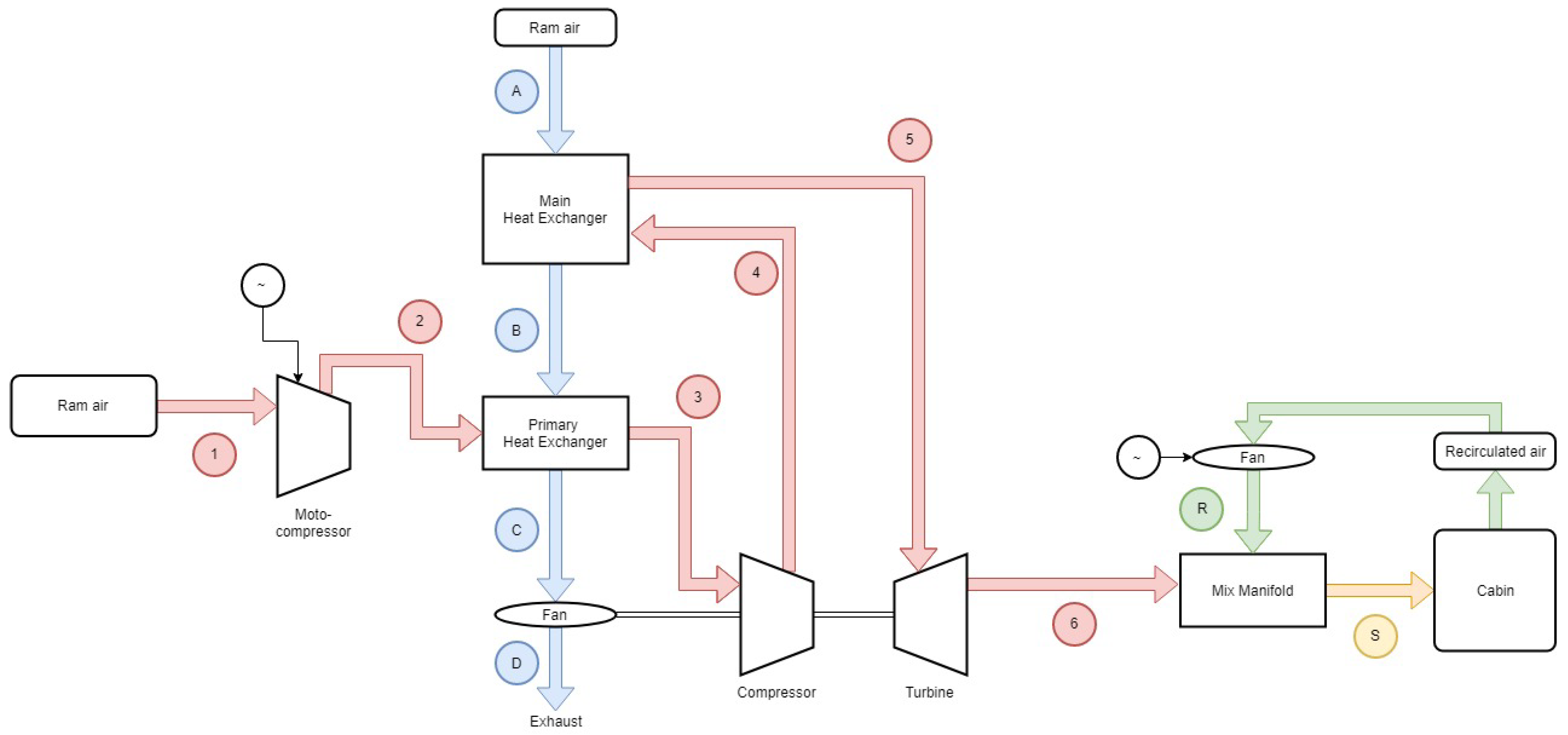
The choice was made here to study an electric architecture, due to the electrification of aircraft. In addition, the architecture studied is simplified to take into account only the main components. An illustrative diagram is provided on Figure 1, by identifying the different airflows by colors. For the main airflow (represented in red), the air is directly taken from the outside via air inlets (Point 1). The outside air is compressed and therefore heated via an electrically operated compressor (Point 2). Then, the air passes through a first exchanger (cooled by outside air represented in blue) to decrease the temperature (Point 3) and then in a second compressor to gain pressure (Point 4). The air then passes through a new exchanger (Point 5) and then through a turbine for expansion (Point 6). Finally, this air can be mixed with recirculated air (represented in green) from the cabin. The objective is to reach the right temperature and pressure characteristics at Point S. The ECS is used to control all the thermal loads and the dehumidification part is not treated in this paper.
2.2. Aircraft Requirements and Sizing Scenarios
To design ECS, specifications for the aircraft are required, including
- the umber of passengers ,
- the dimensions of the aircraft (length, diameter...),
- the flight characteristics (descent speed, re-pressurization...), and
- assumptions on the overall performance of ECS (leaks, efficiency...).
To study the operations of ECS in different flight configurations, different scenarios are considered. The “hot day” scenario is defined as a scenario with maximum temperatures, solar charges, and a maximum number of passengers. Conversely, the “cold day” scenario is a scenario with minimum temperatures, no solar charge and with a minimum number of passengers. A “standard day” scenario is also considered, with ISA temperatures and an average filling rate. For “hot day” and “cold day” cases, the failure of one of the two ECS packs is also considered.
Then, flight altitude will also be considered because it modifies the external conditions but also impacts the internal conditions, such as the control of pressurization. To consider different cases, the altitudes used for the study will therefore be ground level, an intermediate level () and cruising altitude.
2.3. Heat Loads
When studying an air-conditioning system, the first step is to assess heat/thermal loads. Four heat loads can be studied, including
- external thermal loads, which correspond to heat transfers with the external environment by convection and conduction; they can be positive (outside temperature higher than in the cabin) or negative (outside temperature lower than in the cabin);
- the positive metabolic thermal loads, which correspond to the heat given off by passengers and crew;
- solar thermal charges, zero or positive, due to solar flux through the glass surfaces; and
- positive electrical thermal charges, which represent the thermal losses of electrical components in the form of heat.
The total heat loads are the sum of these four components. The following models for the heat loads use the methods in [26].
First, the external thermal loads are determined via Equation (1),
where A is the exchange surface of the aircraft, is the cabin temperature, is the temperature of the exterior surface of the aircraft, and U is the heat transfer coefficient (of the order of for an Airbus A320-type aircraft).
In the same way, the metabolic loads (here for the passengers) are obtained via Equation (2) with the previous notations. In the case of crew members, these values must be multiplied by two due to the physical activity of the crew members:
Then, the solar heat loads are obtained with the glass surface by using Equation (3),
with coefficient for glass transmissivity, coefficient for projecting the glass surface, the glass surface, and the solar flux.
Finally, the electric heat loads are the sum of a fixed component and a component proportional to the number of passengers, with Equation (4),
where is a fixed value, estimated at for the “hot day” and for the “cold day” (for an Airbus A320-type aircraft).
Generally, these thermal loads are evaluated according to the altitude for the different scenarios. For instance, in the case of an Airbus A320-type aircraft using the previous models, the layout of the thermal loads called the “heat loads envelope” is obtained as shown on Figure 2. This diagram shows the heat loads depending on the altitude for different scenarios. “Hot day” and “standard day” scenarios lead to positive values, which correspond to a need for cooling, contrary to the “cold day” scenario. For “hot day” and “cold day” cases, in case of the failure of one of the two packs, other thermal loads are taken into account. They represent the new authorized loads: the cabin temperature is no longer set at 24 °C, and different values are allowed. These characteristics are also indicated on Figure 2.
2.4. Flow Schedule
Once the heat loads have been determined, it is necessary to estimate the maximum airflow required in the different sizing cases. The airflow from ECS has to ensure several functions: pressurization at altitude, repressurization during the descent phase, cooling or heating if necessary and air renewal for the people on board the aircraft. It is therefore necessary to calculate the flow rates required for each of these functions, assuming only the ECS packs are used for cooling and heating, in order to determine the maximum flow required, called the flow schedule.
First, the air renewal rate is obtained from standards to ensure sufficient fresh air for passengers and crew [33]. For instance, for cases without failure, the minimal airflow per passenger is 0.55 lb/min whereas it is 0.40 lb/min in case of failure. For the crew, standards are 10 ft3/min. These data are used to calculate a global mass flow for fresh air.
Then, according to [33], the pressurization flow rate uses exterior and cabin pressures via Equation (5). For the repressurization flow rate, a repressurization rate of 11 mbar/min is considered,
with the cabin pressure, the exterior pressure and the total aircraft leakage surface.
Finally, the air conditioning or heating flows are obtained directly from the thermal loads via Equation (6) (case of cooling),
where is the specific heat capacity and the blown air temperature.
These different flows allow, for each case, to define the flow schedule. The latter is the maximum value between the pressurization and renewal functions. Cooling and heating cases are less critical because it is possible to blow colder/warmer air after the turbine and mix it with recirculated air to achieve the heat load objectives.
Figure 3 represents the flow schedule for the different sizing scenarios. The shaded area corresponds to the values prohibited for flow because pressurization or air renewal are not guaranteed. For instance, in the case of the “cold day” scenario with pack failure, the graph shows that air renewal (blue line) is limiting on the ground while pressurization (green line) is limiting at intermediate and cruise altitudes. Heating (red line) is not considered critical because the blown air temperature can be changed. Thus, the flow schedule (depending on altitude) corresponds to the upper outline of the grey area. For instance, in this example, the sizing scenario is the “hot day” with a pack failure, which leads to a flow schedule of approximately 0.5 kg/s. It is interesting to note that, without considering the cooling/heating assumption given previously, the flow schedule would be sized by the “hot day” scenario without failure with a higher value of approximately 0.9 kg/s.
2.5. Thermodynamic Models
The objective is to calculate the thermodynamic characteristics (temperature, pressure, mass flow) of the different operating points (altitudes and “cold or hot day”). For this, the equations below are used, in the same way as [24].
To model the compressors and the turbines, isentropic transformations associated with an isentropic efficiency are considered. For example, in the case of a compressor supplying power , Equations (7)–(9) are used, noting by I the input and O the output. Equation (8) needs to be modified for a turbine. We have
where T is the real temperature, is the isentropic temperature, P is the pressure, is the isentropic efficiency for the compressor, and is the mass flow.
For fans, the relation (10) is used to calculate the power of the fan . We have
where is the mass flow, is the pressure gain of the fluid, is the density of the input fluid, and is the fan efficiency.
For heat exchangers, perfect exchange between the two fluids, considering no external losses, is assumed. Thus, Equation (11) makes it possible to model the heat transfer between the two fluids, by indicating the two fluids of the heat exchanger by 1 and 2 and keeping the previous notations. We have
Moreover, pressure losses are considered in the heat exchangers, expressed via a difference or a pressure ratio . Equation (12) is used, keeping the previous notations:
3. Modeling: ECS Components
The objective of this part is to define the models used for the main components of ECS. With this in mind, different methodologies can be used. First, many models can be obtained from analytical equations based on physical relationships. Then, scaling laws are useful to define characteristics from a reference [34,35]. Finally, some models can be obtained from surrogate models, via an existing dataset or via numerical simulations to generate this data [36]. For all of the components under study, their mass, their electrical consumption, and their additional drag will be considered.
3.1. Air Inlets
Air inlets are necessary to supply the cabin with air or to cool the heat exchangers. However, it has a cost in terms of consumption. The drag generated by air inlets, as well as the total pressure and mass (due to structural reinforcements), are evaluated in this section. It is considered that air inlets do not consume electrical energy (neglected for the actuated inlet doors) in the first instance.
Different types of air inlets exist (Figure 4). Two families can be distinguished:
- the scoop inlet, which is an emergent inlet that recovers air at high pressure throughout most of the Mach number range but at the cost of high drag; and
- the flush inlet, which is a submerged or “hollowed out in the fuselage” inlet which generates less drag for the air taken off but with little pressure increase.
These air intakes can also have different shapes, which allow different performances. They can for example be rectangular (as shown in Figure 4) or more aerodynamic (NACA air inlets). The objective is to choose the architecture which allows the best tradeoff for drag/pressure performance. Indeed, it is interesting to have a low drag (flush inlet) to minimize consumption but also to have a high-pressure level (scoop inlet) to facilitate the increase in pressure necessary to bring air into the cabin.
Schematic air inlets are shown in Figure 5. Many dimensions can be considered, but to simplify, only the main dimensions have been taken into account, particularly the length of the air intake L ( and on the figure) and its height H ( on the figure).
In the following, some examples are presented for modeling the drag, pressure recovery, and mass of air inlets. Detailed models can be found in [38,39].
3.1.1. Drag
The objective of this section is to obtain models in order to estimate the drag generated by scoop inlets designed with a diverter (Figure 4, scoop inlet). The models for flush inlets are based on a similar methodology.
According to [10], the scoop inlet drag can be calculated by using Equation (13) where is the free-stream velocity, is the free-stream mass flow through the inlet capture area, and is the drag coefficient of the scoop inlet:
The drag coefficient can be estimated by using different abacuses depending on the mass flow ratio , the Mach number , and geometric parameters [10]. A generic model for this coefficient can be obtained by computing a surrogate model that is established by using the variable power law method (VPLM) [40,41] and a design of experiments from abacuses. Computations show that the model can be simplified to a function based on only the two main variables, the Mach number , and the mass flow ratio (obtained by using [10]), and that a polynomial model gives better results than variable power laws. The results of the regression model performed on are shown in Figure 6 and Figure 7. Figure 6 gives the maximum and mean errors and standard deviations for different polynomial models of order 3, considering different numbers of terms. Using more than five terms does not improve the model. Thus, a model with five terms is chosen and given in Equation (14). Lastly, Figure 7 gives two types of information. On the one hand, the figure on the left provides a comparison between the data used (abscissa) and the results obtained with the model (ordinate). A perfect model would result in points located on the blue line. On the other hand, the error distribution is given in the figure on the right. It shows a very small and relatively centered error for the model. We have
As an application, at Ma = 0.8 and = 0.5 kg/s, the models give = 1.89 and a scoop inlet drag of N. Moreover, when the flow is increased to = 1.0 kg/s, the drag increases to = 251 N.
3.1.2. Pressure Recovery
In this section, a methodology to estimate the pressure recovery of the flush inlets is applied. In comparison to drag models, an alternative method is used, based on surrogate models using numerical simulation data. For scoop inlets, the methodology is similar.
The first step is to determine the characteristic variables that allow modeling of total pressure . For this, a dimensional analysis is performed and the Buckingham theorem is used [42,43]. The dimensional analysis allows the total pressure to be related to various physical quantities via an undetermined function f, as presented in Equation (15), where V is the flow velocity, is the density, is the dynamic viscosity, T is the temperature, and r is the specific gas constant. The application of the Buckingham theorem makes it possible to restrict the variables via dimensionless parameters given in Equation (17). It is interesting to note that typical dimensionless numbers such as the Reynolds number or the Mach number can be retrieved (with the air heat capacity ratio). A new relation including only dimensionless parameters is then reexpressed via Equation (16) with another undetermined function g. We have
where:
By using the tool pyVPLM, a design of experiments is generated for these dimensionless numbers. CFD simulations are then performed by using ANSYS Fluent. The boundary conditions are given in Figure 8, and the mesh has been refined in the usual areas (walls, near and downstream of the air inlet) with the size required to ensure the convergence of the results. The assumption of perfect gas has been made. Concerning turbulence, a Realizable model was used and the values of corresponding to the walls were verified. The simulations can be used to produce results similar to those shown in Figure 8, which represents an example of the airflow velocity for one of the simulations performed. It then allows the estimation of the corresponding total pressure value and thus the parameter in each case.
Finally, pyVPLM is used to process the simulation results considering a variable power law for the model to estimate the function g. Considering an order of 3, Figure 9 is obtained and can be used to select the model as for Figure 6. A number of terms equal to 9 is chosen as the best compromise between complexity and accuracy, with a maximal error of 4.7 % and a mean error of 1.3 %. Figure 10 gives more details on the error of the chosen model in a similar way to Figure 7. As a result, Equation (18) is used to estimate and then using Equation (17).
3.1.3. Mass
The integration of an air inlet requires structure modifications around it as well as additional components necessary for its operation (flap, actuators).
In the case of air inlets, scaling laws are considered in this paper to estimate the mass of the latter [44]. The scaling laws can be used to study the effects of a geometric change on the characteristics of a “custom-made” component compared to an existing reference component. For air inlet, its mass can be estimated as a function of the mass flow rate , using Equation (19) proposed in [38], assuming the geometry and the flow characteristics are conserved. Here, the reference mass of the air inlet, for a reference mass flow rate kg/s, is assumed to be kg. We have
3.2. Heat Exchangers
The heat exchangers do not consume electrical energy and add no additional drag. Thus, only their mass is evaluated and pressure drops are assessed.
The heat exchangers under study are cross-flow plate fin-type heat exchangers, which are often used in aeronautics. The shape of the fin mesh can vary. Fins with triangular, sinusoidal or rectangular cross-sections can be found. In this article, triangular cross-sections are chosen. Indeed, these sections have the advantage of being simple to model numerically and of delimiting easily calculable surfaces. Thus, many articles focused on heat exchangers using triangular fins [16,17]. The geometry of one heat exchanger is shown in Figure 11. The air in the ECS pack is represented by exhaust air (or hot air) and the outside air to cool the heat exchanger by fresh air (or cold air). The study can be reduced to an elementary mesh comprising a triangular passage for each of the airflows. Different parameters like the angle of the triangle , the height of the triangles H or the dimensions of the heat exchanger are taken into account.
For each fluid (hot or cold air), the notion of hydraulic (or equivalent) diameter of a triangular half-mesh is introduced to model the flows. It is defined by using Equation (20),
where is the hydraulic diameter, is the cross section, is the perimeter of the cross-section outline, H is the height of the triangle, and is the angle of the triangle.
Once the geometry is known, the objective is to find a method that makes it possible to calculate the dimensions of the heat exchanger knowing the required input and output temperatures, pressures, and mass flows. For this, the number of transfer units (NTU) method is used [45,46]. It can be broken down into several stages:
- models for the Nusselt number and the coefficient of friction using dimensionless numbers;
- calculation of the heat transfer coefficient U;
- calculation of the minimum thermal capacity ;
- calculation of the number;
- calculation of the heat exchanger exchange surface, its dimensions and its mass; and
- calculation of pressure drop
However, an algebraic loop is present because of the dimensions of the heat exchanger. Indeed, an initial reference dimension is needed to estimate the dimensionless numbers. Thus, a reference surface (or a reference length) is initialized and will be recalculated. The objective is to obtain the convergence for this value. Steps 1 to 5 are within the algebraic loop, whereas step 6 can be achieved after the resolution of the algebraic loop.
Following the NTU method, step 1 aims at determining the Nusselt number , which makes it possible to know the convection coefficient h, the latter characterizing heat exchanges near the walls. Similarly, to determine pressure losses, it is necessary to know the friction coefficient f. In this type of application, the Nusselt number can generally be expressed as a function of the Reynolds number and the Prandtl number in forced convection. These dimensionless numbers are defined by using Equation (21),
where is the fluid thermal conductivity and h is the convection coefficient and using the previous notations.
For the case of triangular ducts, the Nusselt number and the friction coefficient are expressed, respectively, with relations (22,23) [16,17]:
Step 2 consists in determining the heat transfer coefficient in order to size the heat exchanger.
First, efficiencies to take into account the conduction effects at the fins have to be calculated. For each fluid, Equation (24) can be used to estimate the efficiency reduced to a single fin ,
where m is a parameter defined by , with the thermal conductivity of the material that constitutes the heat exchanger and the thickness of the separating layers.
Then, Equation (25) is used to estimate overall efficiency [45]. Clogging of the fins is not considered here. We have
where is the surface of separating layers (chosen as reference surface) and S is the surface of the fins in contact with the considered fluid.
Finally, the heat transfer coefficient U can be expressed by using Equation (26) [45,47]. The central term corresponds to conduction between the plates. The other two terms correspond to convection for hot fluid and cold fluid. The calculated efficiencies allow the conduction effects at the fins to be taken into account. We have
where
- is the heat transfer coefficient (relative to the surface );
- and are the convection coefficients for hot fluid and cold fluid;
- and are the surfaces of the fins in contact with hot fluid and cold fluid; and
- and are the efficiencies for conduction in the fins for hot fluid and cold fluid.
Step 3 allows estimating the minimum thermal capacity between the two fluids, noted . The minimum thermal capacity is simply calculated by taking the minimum value for the two fluids of the product .
Step 4 is the calculation of the NTU number. First, two parameters R and P are introduced. For example, if the hot fluid corresponds to the minimum thermal capacity, Equations (27) and (28) define the parameters. The indices H and C correspond, respectively, to the hot fluid and the cold fluid, and the indices i and o correspond, respectively, to the input and output values of the heat exchanger. We have
Then, with these two parameters, the number is obtained by numerically solving the implicit Equation (29), valid for a cross-flow heat exchanger with two unmixed fluids [46]. We have
Lastly, step 5 allows us to obtain the surface (chosen as reference previously) via Equation (30) [46]. This new value makes it possible to iterate the process until convergence. We have
Once convergence has been reached, it is possible to determine the dimensions and the mass of the heat exchanger simply via its geometry and its density.
Finally, for step 6, the pressure drops for each of the two fluids can be evaluated by using Equation (31), thanks to the friction coefficient obtained in step 1. We have
where V is the average velocity of the fluid in the triangular section (obtained from the flow rate and the cross section) and L is the length of the triangular duct (obtained with the heat exchanger dimensions).
3.3. Electric Motors
Electric motors are essential elements to model because of their consumption and their mass. All the models proposed in this article are obtained via scaling laws. For a variable x, is the value defined by . Here, the reference chosen is a high-speed motor from the aeronautical industry. It is a synchronous motor with permanent magnets with one pair of poles and air cooling in forced convection.
The three input variables of the motor model are its diameter , its operating speed and its mechanical power . The following assumptions are made: geometric similarity, identical materials, constant maximum temperature, and fixed convection coefficient.
The newly designed motor mass is obtained via the trivial scaling law . The torque of the motor is estimated by using Equation (32):
The losses and efficiency of this motor can be calculated, and the thermal behavior (losses and heat dissipation) must be verified.
First, for estimating the total losses of the motor, the Joule losses and the iron losses are calculated. The Joule losses limit the torque via the current and the iron losses limit the rotational speed of the motor. Equations (33) and (34), issued from [3,35], are used with and two parameters defined in Equations (35) and (36). We have
where:
As a consequence, the total losses of the motor can be expressed by using Equation (37):
As a consequence, the efficiency of the electric motor is deduced from Equation (38), with the electrical power to be supplied to the electric motor. We have
Moreover, an equation makes it possible to check the maximum temperature. The ratio defined by must remain less than 1 to maintain the maximum temperature less than or equal to that of the reference machine.
As a result, these models can be used in order to estimate the three motor parameters for different applications. It allows for instance optimizing the motor according to its mass or its efficiency for a given power with respect to a diameter ratio and speed.
3.4. Turbomachines
A turbomachine (like a compressor, fan, or turbine) does not directly consume electrical energy and does not generate drag. Thus, only its mass is estimated.
For preliminary sizing, a first solution is to use the NsDs diagram [19,20], which takes the efficiency into account. This solution has the disadvantage of using complex and moderately available abacuses. Another simpler solution, also based on the consideration of efficiency, is the Cordier diagram.
The Cordier diagram represents a curve that connects two dimensionless parameters, characterizing a turbomachine (single stage) having maximum efficiency [21]. These two dimensionless numbers are the dimensionless speed and the dimensionless radius , which are defined by Equations (39) and (40),
where N is the speed of rotation in RPM, w is the specific work, R is the radius of the turbomachine, is the volume flow, and is a constant.
This diagram also indicates the type of machine (axial, centrifugal, etc.) with the best efficiency for a given parameter. It has been updated and simplified recently by [48]. On this diagram, one curve represents compressor-type machines and another one represents turbine-type machines.
In order to compute analytical expressions of these two curves, the VPLM method was used based on reference data from [48]. This type of model is particularly effective when the parameters vary over several decades. The model for compressors is given by Equation (41) and for turbines by Equation (42). The models give a maximum error of 5 % and an average error of less than 2 %. The resulting curves are shown in Figure 12. We have
Thus, from the required performance of a turbomachine (speed, work), its radius R can be obtained by using the previous models. Indeed, from its specifications, Equation (39) gives the dimensionless number . Then, by using Equation (41) (for a compressor), the dimensionless number is obtained. Finally, by using Equation (40), the radius can be estimated.
From this radius, the mass M is estimated by using a scaling law (43) from a reference indexed , in the same way as in the previous part:
3.5. Other Models for Mass
The two ECS packs, made up of the different components detailed above (excluding air inlets), must be integrated on the aircraft. Additional parts (casing, structural reinforcements, pipes, valves) are then necessary. To take into account these elements, an oversizing coefficient is considered. In this work, the mass of the components of the pack is multiplied by a factor of 1.5 (obtained from industrial data analysis) to calculate the mass of the pack once integrated.
A network of ducts is used to distribute the air into the aircraft. The mass of this network is important and constitutes the main mass of the complete ECS system. An estimation model is given in Equation (44) as a function of the number of passengers and the number of engines . This is an empirical model from FAST-OAD, an overall aircraft design platform developed by ISAE-SUPAERO and ONERA [49]. It has been adapted from a model for conventional ECS (calibrated on an Airbus A320 aircraft), identifying the terms that correspond to the different masses of the system (engine bleed air system, conventional packs, network of ducts). We have
Therefore, the total mass of the system is the sum of three terms: the mass of the two packs, the mass of the air inlets and the mass of the network of ducts.
4. Results and Discussion: Architecture Sizing and Optimization
The objective of this section is to achieve an application for an ECS sizing based on the models presented in this paper. In particular, the sizing method as well as the results and discussions are presented.
4.1. Fuel Consumption Models
Before sizing the electric ECS architecture, some additional models are needed. Indeed, adding an electric system to an aircraft increases fuel consumption. This increase can have three different causes: an increase in mass, additional drag, or additional electrical (or mechanical) consumption. This additional mass of fuel can be estimated by using Equation (45) [50], also used in [38]:
where
- is the mass of the system;
- is the additional drag due to the system;
- is the additional electrical power which must be consumed;
- f is the lift-to-drag ratio, such as ;
- is the specific fuel consumption;
- g is the acceleration of terrestrial gravity such that ;
- t is the duration of the flight phase;
- is the efficiency of electric generators (on the turbojet); and
- is the coefficient for characterizing the fuel flow consumed per amount of mechanical energy produced.
In order to obtain more accurate results, other more detailed models can be used [30], especially for shaft power off-takes [51]. Moreover, the flight can be divided into different phases in order to obtain constant lift-to-drag ratio and specific consumption values over this phase. For instance, the following phases can be chosen: ground, take-off, climb, cruise, descent, and landing.
4.2. Methods
A sizing and optimization process is defined for the electric ECS. The CeRAS aircraft is taken as an application case [29]. The latter is a reference aircraft in the scientific literature and is comparable to the Airbus A320 or Boeing B737. In order to obtain reasonable size motor compressors, two motor compressors per pack are considered for this type of aircraft.
The objective is to minimize the fuel consumption of the system estimated by using the previous models. Due to the complexity of the ECS specific models, especially due to the interactions and couplings between the different components of the ECS system, a MDAO approach is adopted. A monolithic approach, based on a single optimizer, is used and the resolution of multidisciplinary couplings is based on IDF and NVH formulations [7]. The optimization is performed by using a genetic algorithm (NSGA-II [52]). Even if numerous methods can be adapted to solve such problems [53,54], this method has two main advantages. On the one hand, it allows providing a result despite the exploration of nonphysical areas generating numerical problems. On the other hand, this type of algorithm is particularly adapted to deal with nonconvex problems with local optimums, which is most probably the case of the considered problem because of its complexity.
The XDSM and DSM diagrams of the ECS sizing process are given in Figure 13 and Figure 14. The XDSM diagram allows us to visualize the formulation of the optimization problem, whereas the DSM diagram allows us to represent in detail the interactions between the different disciplines. The green blocks represent the different calculation modules. The input parameters of a module are represented on the vertical lines whereas the output parameters are on the horizontal lines.
These two diagrams allow us to identify the interactions between the different disciplines and the possible algebraic loops. The optimization problem (46) contains 27 optimization variables and 28 constraints. Initially, the sizing problem included seven multidisciplinary couplings and thus seven algebraic loops. Thanks to the IDF and NVH formulations, these algebraic loops have been eliminated as shown in the diagrams.
where are mass flows, are temperatures, are compression/expansion ratios, and are widths and heights of heat exchanger ducts, and are efficiencies of heat exchangers, and are the variables for checking the motor cooling. and are normalized consistency variables for heat exchangers pressure drops and lengths. and are the associated estimated variables that are used in the consistency constraints with respect to the NVH formulation.
The sizing of the ECS is performed in two steps. In the first step, an architecture sizing is performed for the different sizing scenarios. These are based on the “hot day” and “cold day” scenarios, with and without failure of one of the two ECS packs, by considering two characteristic flight phases (cruise and ground). This step allows defining the maximum characteristics of the various components and the total mass of the system: it is thus an approach that leads to a possible oversizing of the system. In the second step, the system is optimized for average flight conditions. This allows the evaluation of the performance of the system (electrical power consumption, generated drag) and its corresponding fuel consumption.
4.3. Results and Discussion
Before detailing the main results, some elements concerning the numerical solution of the optimization problem are provided. For each sizing, the optimization problem has been run and solved offline on a typical scientific laptop with a computation time of approximately 10 minutes.
For illustrating convergence results for the optimization problem, the “standard day” scenario in cruise without failure is considered. The genetic algorithm has been parameterized with 2 × 10⁵ generations. Figure 15 shows the raw data for each generation considered as successful, i.e., that has been computed successfully (absence of NaN values) and whose absolute relative error is less than 1000 % with respect to the final value obtained for the objective. The configurations which do not respect the constraints (defined as unfeasible) are represented in red, whereas the ones which respect the constraints (defined as feasible) are in blue. It is interesting to note the difficulty of finding a feasible solution for the first generations and the step-by-step convergence of feasible solutions after 0.75 × 10⁵ generations. To emphasize this, a postanalysis shows that for the 2 × 10⁵ generations, the repartition of solution cases yields 1.74 % of NaN, 39.18 % of absolute relative errors greater than 1000 %, 54.04 % of unfeasible, and 5.04 % of feasible. The raw data is postprocessed on Figure 16 demonstrating the convergence. Indeed, the moving average of the absolute relative error for the successful cases (in blue), considering consecutive values, stabilizes after 1 × 10⁵ generations. The difficulty for the genetic algorithm to find successful solutions is particularly visible between 0.25 × 10⁵ and 0.75 × 10⁵ generations. Moreover, the best lowest value for the feasible solutions (in orange) converges to the optimal solution.
Concerning the results of the optimization process, for illustrating the first step, the sizing scenario “hot day” with a failure of one of the two packs during cruise is considered. The sizing results in the set of system parameters. For example, an airflow of 0.5 kg/s is obtained for the ACM, with a cooling flow of 0.46 kg/s for the exchangers. The power of the electric compressors is 80 kW with a compression ratio of 4.15. The recirculation fan has a power of 16 kW for an airflow of 0.25 kg/s. Finally, the mass of the exchangers is 60 kg.
The main characteristics of the ECS (for one pack) for the different sizing scenarios are given in Table 1. The scenarios that allow sizing the mass of one of the components are indicated in the last column. This means that the maximum mass of one of the components was obtained for these scenarios. It is interesting to note that many of the sizing scenarios are critical for sizing. This approach results in a total mass of around 1500 kg for the ECS: 390 kg for each of the two packs, 150 kg for the air inlet assembly, and 570 kg for the network of ducts.
Several remarks can be made. First of all, the sizing is complex to perform numerically in the “cold day” scenarios in cruise because of the low outside temperatures: the airflow of the ACM tries to bypass the exchangers. Similarly, in the case of waiting on the ground, the optimizer seeks to minimize the system’s electrical power consumption at the cost of a large increase in mass. These cases therefore require additional constraints to be added to the optimization problem. Finally, for some scenarios, the sizing results in a mass flow rate supplied to the ACM that is greater than the minimum required flow rate (flow schedule), in order to minimize fuel consumption.
In a second step, for evaluating the average performance of the ECS, a sizing is performed for the “standard day” scenario in cruise phase without failure of one of the two packs. In this case, the complete system (including the two packs) consumes 190 kW of electrical power, 95% of which is due to the electric compressors. It also generates 200 N of drag: 64% from the scoop air inlets for the ACM and 36% from the flush air inlets for cooling the heat exchangers. The corresponding airflow rates are 0.28 kg/s and 0.22 kg/s, respectively. The airflow rate for the recirculation of air from the cabin is 0.25 kg/s.
These different data allow for estimating the average fuel consumption due to the ECS. The fuel consumption per hour of the system in the average case is 88 kg/h. The breakdown of the fuel consumption is given in Figure 17 via a Sankey diagram which allows us to represent the different energy flows and their schematic use. The thermal losses for the electric power are not detailed in the figure to focus on the main flows between components. Overall, the following distribution is obtained: 48% for the electrical power consumption (mainly electric compressors), 10% for the generated drag, and 42% for the mass of the complete system. The minimization of the fuel consumption of the system is not simply a matter of minimizing the mass of the system, but a complex global optimization including particularly the electrical power consumption.
For comparison, in the case of the “hot day” scenario during cruise without a pack failure, the fuel consumption per hour of the system is 106 kg/h. In the case of waiting on the ground without a pack failure, the consumption per hour, only due to electrical power consumption, is 19 kg/h for the “standard day” and 47 kg/h for the “hot day”.
The sizing process proposed in this article thus allows a quick estimation of the main characteristics of the electric ECS. To perform a more accurate optimization of the system, it would be necessary to perform a single multipoint optimization that simultaneously integrates and verifies the performance of the system for each operating point. However, this much more complex approach would require detailed industrial and operational data, particularly on the frequency of encounters of the different flight and operating conditions of the ECS system.
5. Conclusions
In this paper, an electric ECS architecture has been modeled, sized, and optimized. A major contribution of this paper concerns the development of multiple models for all the components of the system, by adopting various modeling approaches. The other main contribution deals with the formulation and resolution of the optimization problem for the ECS in order to proceed with an application to estimate the impact in terms of system weight, power, and fuel consumption on a reference aircraft.
More specifically, different methods and models have been presented. First, methods to determine the flow schedules of an ECS have been presented. Moreover, methods and models for sizing the main components such as air inlets, heat exchangers, turbomachines, and electric motors have been detailed. These models are of different type such as scaling laws, empirical laws, analytical and surrogate models. Then, a method for sizing and optimizing at the aircraft level an electric architecture for the ECS has been detailed. It contains initially seven multidisciplinary couplings that are solved using IDF and NVH approaches. Finally, the optimization problem consists of 24 optimization variables and 42 constraints.
Results show that each scenario yields different optimal designs for the system. Most of them are sizing cases for one of the components. Once the extreme cases for the components are obtained, the system is optimized for the standard day scenario. Therefore, the optimal ECS accounts for around 200 N of drag, 190 kW of electric power and 1500 kg of mass for the CeRAS reference aircraft.
Although this paper has made it possible to achieve a preliminary sizing of an electric ECS, some limitations are to be mentioned and open perspectives for future developments. For example, the presented models could be improved, especially concerning turbomachines. Moreover, a single architecture has been considered in this paper. It would be interesting to perform multiple sizing on conventional and electric architectures, with and without VCS, in order to compare the performance and especially the fuel consumption. This would require the development of specific engine models for conventional pneumatic architectures, but also generic codes to test multiple configurations.
Author Contributions
Conceptualization, T.P. and S.D.; formal analysis, T.P. and S.D.; methodology, T.P.; software, S.D.; writing—original draft preparation, T.P.; writing—review and editing, S.D., V.P.-B., and E.B. All authors have read and agreed to the published version of the manuscript.
Funding
This research received no funding. This study is supported by ISAE-SUPAERO, within the framework of the research chair CEDAR (Chair for Eco-Design of AiRcraft).
Data Availability Statement
The data presented in this study are available on request from the corresponding author.
Acknowledgments
The authors would like to thank David Lavergne for his relevant feedback.
Conflicts of Interest
The authors declare no conflict of interest.
Abbreviations
The following abbreviations are used in this manuscript:
| ACM | Air Cycle Machine |
| CFD | Computational Fluid Dynamics |
| ECS | Environmental Control System |
| IDF | Individual Discipline Feasible |
| IPS | Ice Protection System |
| MDAO | Multidisciplinary Design Analysis and Optimization |
| MEA | More Electric Aircraft |
| NTU | Number of Transfer Units |
| NVH | Normalized Variable Hybrid |
| VCS | Vapor Cycle System |
| XDSM | eXtended Design Structure Matrix |
References
- Chakraborty, I.; Trawick, D.; Mavris, D.; Emeneth, M.; Schneegans, A. Integrating Subsystem Architecture Sizing and Analysis into the Conceptual Aircraft Design Phase. In Proceedings of the 4th Symposium in Collaboration in Aircraft Design, Toulouse, France, 25–27 November 2014. [Google Scholar]
- Maré, J.C. Aerospace Actuators 3: European Commercial Aircraft and Tiltrotor Aircraft; John Wiley & Sons: Hoboken, NJ, USA, 2018. [Google Scholar] [CrossRef]
- Delbecq, S. Knowledge-Based Multidisciplinary Sizing and Optimization of Embedded Mechatronic Systems—Application to Aerospace Electro-Mechanical Actuation Systems. Ph.D. Thesis, INSA, Toulouse, France, 2018. [Google Scholar]
- Kroo, I.; Altus, S.; Braun, R.; Gage, P.; Sobieski, I. Multidisciplinary optimization methods for aircraft preliminary design. In Proceedings of the 5th Symposium on Multidisciplinary Analysis and Optimization, Panama City Beach, FL, USA, 7–9 September 1994; p. 4325. [Google Scholar] [CrossRef]
- Perez, R.; Liu, H.; Behdinan, K. Evaluation of multidisciplinary optimization approaches for aircraft conceptual design. In Proceedings of the 10th AIAA/ISSMO Multidisciplinary Analysis and Optimization Conference, Albany, NY, USA, 30 August–1 September 2004; p. 4537. [Google Scholar] [CrossRef]
- Martins, J.R.; Lambe, A.B. Multidisciplinary design optimization: A survey of architectures. AIAA J. 2013, 51, 2049–2075. [Google Scholar] [CrossRef]
- Delbecq, S.; Budinger, M.; Reysset, A. Benchmarking of monolithic MDO formulations and derivative computation techniques using OpenMDAO. Struct. Multidiscip. Optim. 2020, 62, 645–666. [Google Scholar] [CrossRef]
- Herzog, J. Electrification of the environmental control system. In Proceedings of the 25th International Congress of the Aeronautical Sciences, Hamburg, Germany, 3–8 September 2006; pp. 1–4. [Google Scholar]
- Lawson, C.P. Environmental control systems. In Encyclopedia of Aerospace Engineering; John Wiley & Sons, Ltd.: Chichester, UK, 2010. [Google Scholar] [CrossRef]
- ESDU (Engineering Sciences Data Unit). ESDU 86002: Drag and Pressure Recovery Characteristics of Auxiliary Air Inlets at Subsonic Speeds; Technical report; ESDU: London, UK, 1986. [Google Scholar]
- Devine, R.; Watterson, J.; Cooper, R. An investigation into improving the performance of low speed auxiliary air inlets using vortex generators. In Proceedings of the 20th AIAA Applied Aerodynamics Conference, St. Louis, MO, USA, 24–26 June 2002; p. 3264. [Google Scholar] [CrossRef]
- Stalewski, W.; Żółtak, J. The preliminary design of the air-intake system and the nacelle in the small aircraft-engine integration process. Aircr. Eng. Aerosp. Technol. Int. J. 2014, 86, 250–258. [Google Scholar] [CrossRef]
- da Silveira, B.; Souza, P.; Almeida, O. Numerical investigation of a NACA air intake for a canard type aircraft. Int. J. Adv. Eng. Res. Sci. 2017, 4, 237158. [Google Scholar] [CrossRef]
- Almeida, O.d.; Souza, P.C.; Cunha, E. A Numerical Approach for Implementing Air Intakes in a Canard Type Aircraft for Engine Cooling Purposes. J. Aerosp. Technol. Manag. 2021, 13, 1–18. [Google Scholar] [CrossRef]
- Sanchez, F.; Delbecq, S.; Budinger, M.; Hazyuk, I. Modelling and design approaches for the preliminary design of power electronic converters. In Proceedings of the ELECTRIMACS, Toulouse, France, 4–6 July 2017. [Google Scholar]
- Zhang, L.Z. Numerical study of periodically fully developed flow and heat transfer in cross-corrugated triangular channels in transitional flow regime. Numer. Heat Transf. Part Appl. 2005, 48, 387–405. [Google Scholar] [CrossRef]
- Liang, C.; Tong, X.; Lei, T.; Li, Z.; Wu, G. Optimal design of an air-to-air heat exchanger with cross-corrugated triangular ducts by using a particle swarm optimization algorithm. Appl. Sci. 2017, 7, 554. [Google Scholar] [CrossRef]
- Vargas, J.V.; Bejan, A. Thermodynamic optimization of finned crossflow heat exchangers for aircraft environmental control systems. Int. J. Heat Fluid Flow 2001, 22, 657–665. [Google Scholar] [CrossRef]
- Balje, O. A study on design criteria and matching of turbomachines: Part A– Similarity relations and design criteria of turbines. J. Eng. Power 1962, 84, 83–102. [Google Scholar] [CrossRef]
- Balje, O. A study on design criteria and matching of turbomachines: Part B — Compressor and pump performance and matching of turbocomponents. J. Eng. Power 1962, 84, 103–114. [Google Scholar] [CrossRef]
- Cordier, O. Ähnlichkeitsbedingungen für Strömungsmaschinen. BWK Bd 1953, 6, 337–340. [Google Scholar]
- Tartousi, H. Simulation Numérique des Compresseurs et des Turbines Automobiles. Ph.D. Thesis, Ecole Centrale de Lyon, Lyon, France, 2011. [Google Scholar]
- Smith, A.; Childs, T.; Chen, R. Study into electrically shaft driven air cycle machines. In 1st International Conference on Advances in Aerospace Structures, Systems and Technology; Croydon: London, UK, 2018. [Google Scholar]
- Santos, A.; Andrade, C.; Zaparoli, E.L. A thermodynamic study of air cycle machine for aeronautical applications. Int. J. Thermodyn. 2014, 17, 117–125. [Google Scholar] [CrossRef]
- Sielemann, M. Device-Oriented Modeling and Simulation in Aircraft Energy Systems Design; Technische Universität Hamburg: Hamburg, Germany, 2012. [Google Scholar] [CrossRef]
- Tfaily, A.; Kokkolaras, M. Integrating air systems in aircraft multidisciplinary design optimization. In Proceedings of the 2018 Multidisciplinary Analysis and Optimization Conference, Atlanta, GA, USA, 25–29 June 2018; p. 3742. [Google Scholar] [CrossRef]
- Devadurgam, H.; Rajagopal, S.; Munjulury, R.C. Analytical Design and Estimation of Conventional and Electrical Aircraft Environmental Control Systems. engrXiv 2019. [Google Scholar] [CrossRef]
- Crabé, C.; Joksimovic, A.; Benichou, E.; Carbonneau, X. A Methodology to Evaluate Electric Environmental Control System Impact on Aircraft Drag and Mission Performance. In Proceedings of the AIAA Aviation 2019 Forum, Dallas, TX, USA, 17 June 2019; p. 2803. [Google Scholar] [CrossRef]
- Risse, K.; Schäfer, K.; Schültke, F.; Stumpf, E. Central Reference Aircraft data System (CeRAS) for research community. CEAS Aeronaut. J. 2016, 7, 121–133. [Google Scholar] [CrossRef]
- Scholz, D. DOCsys—A method to evaluate aircraft systems. In Proceedings of the Bewertung Von Flugzeugen, the Workshop of DGLR Department of Aerospace Systems, München, Germany, 26–27 October 2018. [Google Scholar]
- Houghton, E.; Carpenter, P.; Collicitt, S.H.; Valentine, D.T. Aerodynamics for Engineering Students, 7th ed.; Elsevier: Amsterdam, The Netherlands, 2017. [Google Scholar]
- Drela, M. Flight Vehicle Aerodynamics; MIT Press: Cambridge, MA, USA, 2014. [Google Scholar]
- Lavergne, D. Model and Sizing Air Systems—Overall Air System Functions, Requirements and Physiological Thresholds; ISAE-Supaero: Toulouse, France, 2020. [Google Scholar]
- Budinger, M.; Liscouët, J.; Multon, B. Chaînes de transmission de puissance mécatroniques-Mise en place des modèles d’estimation pour la conception préliminaire. Techniques de l’Ingénieur. 2011. Available online: https://hal.science/hal-02191712 (accessed on 7 December 2022).
- Budinger, M.; Liscouët, J.; Multon, B. Chaînes de transmission de puissance mécatroniques-Modèles d’estimation. Techniques de l’Ingénieur. 2013. Available online: https://hal.science/hal-01756784 (accessed on 7 December 2022).
- Sanchez, F. Génération de Modèles Analytiques pour la Conception Préliminaire de Systèmes Multi-Physiques: Application à la Thermique des Actionneurs et des Systèmes Électriques Embarqués. Ph.D. Thesis, Université de Toulouse, Toulouse, France, 2017. [Google Scholar]
- Air Inlet of Conditionning Packs of Boeing 787. 2013. Available online: https://commons.wikimedia.org/wiki/File:Air_inlet_of_conditionning_packs_of_Boeing_787.jpg (accessed on 7 December 2022).
- Planès, T.; Habrard, V.; Delbecq, S.; Pommier-Budinger, V.; Benard, E. Thermal management system models for overall aircraft design. In Proceedings of the AIAA AVIATION 2021 FORUM, Virtual, 2–6 August 2021; p. 2428. [Google Scholar] [CrossRef]
- Planès, T. Du Dimensionnement de Systèmes et D’Architectures en Conception Avion à la Simulation de Scénarios Prospectifs Durables pour le Transport Aérien. Ph.D. Thesis, ISAE-SUPAERO, Toulouse, France, 2022. [Google Scholar]
- Sanchez, F.; Budinger, M.; Hazyuk, I. Dimensional analysis and surrogate models for the thermal modeling of Multiphysics systems. Appl. Therm. Eng. 2017, 110, 758–771. [Google Scholar] [CrossRef]
- De Giorgi, F.; Budinger, M.; Hazyuk, I.; Reysset, A.; Sanchez, F. Reusable Surrogate Models for the Preliminary Design of Aircraft Application Systems. AIAA J. 2021, 59, 2490–2502. [Google Scholar] [CrossRef]
- Holmes, M.H. Dimensional Analysis. In Introduction to the Foundations of Applied Mathematics; Springer: Berlin/Heidelberg, Germany, 2009; Volume 56. [Google Scholar] [CrossRef]
- Van Groesen, E.; Molenaar, J. Continuum Modeling in the Physical Sciences; Society for Industrial and Applied Mathematics: Philadelphia, PA, USA, 2007. [Google Scholar] [CrossRef]
- Budinger, M.; Liscouët, J.; Hospital, F.; Maré, J. Estimation models for the preliminary design of electromechanical actuators. Proc. Inst. Mech. Eng. Part J. Aerosp. Eng. 2012, 226, 243–259. [Google Scholar] [CrossRef]
- Incropera, F.; DeWitt, D.; Bergman, T.; Lavine, A. Fundamentals of Heat and Mass Transfer; John Wiley & Sons: New York, NY, USA, 1990. [Google Scholar]
- Navarro, H.; Cabezas-Gomez, L. Effectiveness-NTU computation with a mathematical model for cross-flow heat exchangers. Braz. J. Chem. Eng. 2007, 24, 509–521. [Google Scholar] [CrossRef]
- Kays, W.M.; London, A.L. Compact Heat Exchangers; McGraw-Hill New York: New York, NY, USA, 1958; Volume 196. [Google Scholar] [CrossRef]
- Wolf, D. Das Cordier-Diagramm unter besonderer Berücksichtigung der axialen Turboarbeitsmaschine; Technischen Universität Wien: Vienna, Austria, 2009. [Google Scholar]
- David, C.; Delbecq, S.; Defoort, S.; Schmollgruber, P.; Benard, E.; Pommier-Budinger, V. From FAST to FAST-OAD: An open source framework for rapid Overall Aircraft Design. In Proceedings of the IOP Conference Series: Materials Science and Engineering; IOP Publishing: Bristol, UK, 2021; Volume 1024, p. 012062. [Google Scholar] [CrossRef]
- Moir, I.; Seabridge, A. Design and Development of Aircraft Systems; John Wiley & Sons: Hoboken, NJ, USA, 2012; Volume 67. [Google Scholar] [CrossRef]
- Scholz, D.; Seresinhe, R.; Staack, I.; Lawson, C. Fuel consumption due to shaft power off-takes from the engine. In Proceedings of the 4th International Workshop on Aircraft System Technologies, TUHH, Hamburg, Germany, 23–24 April 2013. [Google Scholar] [CrossRef]
- Deb, K.; Pratap, A.; Agarwal, S.; Meyarivan, T. A fast and elitist multiobjective genetic algorithm: NSGA-II. IEEE Trans. Evol. Comput. 2002, 6, 182–197. [Google Scholar] [CrossRef]
- Kim, H.M.; Michelena, N.F.; Papalambros, P.Y.; Jiang, T. Target cascading in optimal system design. J. Mech. Des. 2003, 125, 474–480. [Google Scholar] [CrossRef]
- Fazlyab, M.; Paternain, S.; Preciado, V.M.; Ribeiro, A. Interior Point Method for Dynamic Constrained Optimization in Continuous Time. In Proceedings of the 2016 American Control Conference (ACC), Boston, MA, USA, 6–8 July 2016; pp. 5612–5618. [Google Scholar] [CrossRef]
Figure 1.
Diagram of the ECS architecture studied.

Figure 2.
Heat loads envelope for an Airbus A320-type aircraft.

Figure 3.
Flow Schedule for an Airbus A320-type aircraft for the different sizing scenarios.

Figure 4.
Air inlets of a Boeing 787 [37].
Figure 4.
Air inlets of a Boeing 787 [37].


Figure 6.
Output of regression model performed on —errors and standard deviation.

Figure 7.
Output of regression model performed on —validation and error distribution.

Figure 8.
Example of results for flow velocity for a flush inlet using ANSYS Fluent.

Figure 9.
Output of regression model performed on —errors and standard deviation.

Figure 10.
Output of regression model performed on —validation and error distribution.

Figure 11.
Chosen geometry for the heat exchanger [16].
Figure 11.
Chosen geometry for the heat exchanger [16].

Figure 12.
Cordier diagram with models and reference points.

Figure 13.
XDSM diagram for the electric ECS sizing.

Figure 14.
DSM diagram for the interactions between electric ECS disciplines.

Figure 15.
Absolute relative errors compared to the optimal value for successful generations.

Figure 16.
Convergence plot with moving average and lowest absolute relative errors.

Figure 17.
Sankey diagram of the energy consumption induced by the electric ECS.


Table 1.
Main results of ECS sizing for the sizing scenarios.
| Sizing Scenario | [kg/s] | [kg/s] | [kg/s] | Drag [N] | Power [kW] | Sizing for the Mass |
|---|---|---|---|---|---|---|
| Cruise Hot day Without failure | 0.33 | 0.38 | 0.31 | 141 | 127 | ✓ |
| Cruise Cold day Without failure | 0.21 | 0.06 | 0.31 | 57 | 71 | ✓ |
| Cruise Hot day With failure | 0.5 | 0.46 | 0.25 | 196 | 176 | ✓ |
| Cruise Cold day With failure | 0.27 | 0.19 | 0.25 | 93 | 79 | |
| Ground Hot day Without failure | 0.41 | 0.58 | 0.49 | 0 | 105 | |
| Ground Cold day Without failure | 0.33 | 0.31 | 0.31 | 0 | 65 | ✓ |
| Ground Hot day With failure | 0.5 | 0.65 | 0.52 | 0 | 156 | ✓ |
| Ground Cold day With failure | 0.34 | 0.26 | 0.28 | 0 | 66 |
Disclaimer/Publisher’s Note: The statements, opinions and data contained in all publications are solely those of the individual author(s) and contributor(s) and not of MDPI and/or the editor(s). MDPI and/or the editor(s) disclaim responsibility for any injury to people or property resulting from any ideas, methods, instructions or products referred to in the content. |
© 2023 by the authors. Licensee MDPI, Basel, Switzerland. This article is an open access article distributed under the terms and conditions of the Creative Commons Attribution (CC BY) license (https://creativecommons.org/licenses/by/4.0/).
Share and Cite
MDPI and ACS Style
Planès, T.; Delbecq, S.; Pommier-Budinger, V.; Bénard, E. Modeling and Design Optimization of an Electric Environmental Control System for Commercial Passenger Aircraft. Aerospace 2023, 10, 260. https://doi.org/10.3390/aerospace10030260
AMA Style
Planès T, Delbecq S, Pommier-Budinger V, Bénard E. Modeling and Design Optimization of an Electric Environmental Control System for Commercial Passenger Aircraft. Aerospace. 2023; 10(3):260. https://doi.org/10.3390/aerospace10030260
Chicago/Turabian StylePlanès, Thomas, Scott Delbecq, Valérie Pommier-Budinger, and Emmanuel Bénard. 2023. "Modeling and Design Optimization of an Electric Environmental Control System for Commercial Passenger Aircraft" Aerospace 10, no. 3: 260. https://doi.org/10.3390/aerospace10030260
Note that from the first issue of 2016, this journal uses article numbers instead of page numbers. See further details here.