The Influence of the Initial Condition in the Transient Thermal Field Simulation Inside a Wall


Institute of Architectural Engineering, Faculty of Civil Engineering, Technical University of Kosice, 042 00 Kosice, Slovakia
*
Author to whom correspondence should be addressed.
Buildings 2019, 9(8), 178; https://doi.org/10.3390/buildings9080178
Submission received: 5 July 2019
/
Revised: 25 July 2019
/
Accepted: 26 July 2019
/
Published: 31 July 2019
(This article belongs to the Special Issue Responsive Architecture)
Abstract
:The envelope structures of buildings are exposed to heat-humidity conditions. The heat and humidity flow through these structures depends on the boundary conditions of the indoor and outdoor environments. This paper shows different initial conditions for the determination of temperature spread. The aim is to bring certain results of temperature calculated considering the initial conditions. When temperature changes, heat flow also rapidly changes. In certain specific cases, it is necessary to consider the initial conditions of temperature—for example; when transient energy simulations of real buildings are carried out. The reasons as to why it is necessary to consider the initial conditions, are shown in the examples of one-layer assemblies. The test walls exposed to the transient hygrothermal conditions are placed in the outdoor test cell. The cell has a stable temperature and relative humidity, and outdoor weather conditions change. The measured data on these walls and the calculated values of the temperatures in the wall structure, according to the different initial conditions, are compared. The average difference of the mean by the simulation and the measured values is significant. For a simulation time of about five days, the initial condition for calculating the temperature in the center of the masonry is necessary.
1. Introduction
We need to know the most exact situation of the initial boundary conditions for the calculation before we begin the computational simulation process. Analytical expressions, constants, or interpolation files are entered together with the properties of structural materials as input data, to determine the simulation criteria, initial conditions, and boundary settings [1,2]. Equilibrium simulation could calculate the distribution of internal air flow, distribution of air temperature and humidity in the room. These values are set as the initial transition analysis conditions [3]. A correct estimate of the initial conditions can have a significant impact on the predicted solutions as well as the overall actual condition of the building [4]. Initial temperature and air humidity must be specified when analyzing building constructions using simulation tools. The impact of the initial moisture content on the hygrothermal behavior of the building is investigated by many authors. The constant temperature of the built-in material in the building structure is generally considered to be the initial state of a rapidly changing factor. However, many simulation calculation tools use the initial temperature as a course of measured or predicted values. The aim is to show the importance of the preliminary calculation in the simulation process and the influence of the calculation on the temperature of the different types of building envelope materials. The preliminary calculation and its impact on the results of the simulation is compared to the measured temperature data, which is recorded in the experimental peripheral wall sections of the external test chamber. Numerical thermal field simulation is a calculation method used to obtain predictive temperature data that is validated using measured data in situ. In particular, the difference in measured and calculated temperature course values over time is quantified, depending on the determination of the initial temperature condition. The difference is influenced by the length of the analysed period.
As stated, the initial state of the transition temperature simulation typically represents the initial temperature distribution throughout the body profile at the beginning of the heat transfer process (t = 0). There are several ways to consider the initial value of the temperature in the structure according to its layout in the profile. The simplest assignment of simulation conditions is the use of a constant temperature across the analyzed component. A more accurate assignment of the initial conditions at t = 0 is the application of the measured temperature profile. Precise information on the temperature profile is rarely provided, so it is therefore appropriate to specify the initial state numerically. The temperature, thus determined, is calculated using the known standing ambient temperatures before time t = 0 or using a known transient temperature (initial pre-calculation). Mathematically, initial conditions are problems due to forward or inverse heat conduction. Problems with forward heat management aim to determine the temperature range of the medium, when the boundaries and initial conditions—the heat source / sink term (if any)—and the physical properties of the material are known [5]. On the other hand, the problem of inverse heat conduction concerns the estimation of the unknown initial temperature distribution, from the knowledge of the measured temperatures or the heat flux at time t > 0 [6]. In this study, the use of thermal initial conditions is demonstrated using numerical examples of simple structures—particularly experimental external test walls. Validation of the simulation is a valuable tool for checking the accuracy of numerical experiments. Outdoor test cells or climate chambers laboratories are suitable for such experiments, and our institution has already carried out similar research. The structure of state status monitoring under transient boundary conditions is the current trend in construction research [7]. An example of an experimental device for monitoring the physical properties of structures is a laboratory climate chamber, which has a “guarded” hot box [8]. Measurements can be made in existing buildings under conditions of use as described in [9]. In practice, it has proved difficult to measure all required inputs at the level required to obtain reliable performance estimates of components in real buildings [10]. Appropriate equipment—thanks to a controlled indoor environment—is an external test cell for the energy and hygrothermal assessment of structures and is for example implemented in Cottbus, Dübendorf, Glasgow, Limelette, Almería, Espoo, Delft, etc. Since 1993, outdoor test cells [11,12] have been employed in a wide variety of applications, from in-situ laboratory testing to complex building testing [12]. Cells are, among other things, useful for laboratory measurements of thermal comfort and emission efficiency, which are important factors in selecting heat emission systems in buildings with a low energy consumption, according to Kurnitski et al. [13]. Other institutes have extensive outdoor laboratories for research on buildings. They mainly focus on green architecture, green roofs and wooden lightweight building envelopes [14]. Another important point of focus in the field of building physics is the overheating of the building in summer. Outdoor monitoring devices as full-scale test cells could also be useful [15].
Accordingly, the external test cells were designed to: (i) form measurement data for hygrothermal reactions of the building envelope components in real climatic conditions in situ; and (ii) to form a validation data set for heat-air-moisture (HAM) simulations [10,16,17,18]. In the paper, the obtained test cell data are used to demonstrate their utility for initial and boundary applications when verifying dynamic simulations.
In order to work with the measured data, local climatic data should be collected at the location of the test cells in the exterior. The weather data used for the numerical calculation can be divided into: (i) typical weather data, (ii) weather data for project purposes, and (iii) weather data for individual investigations. In order to create a typical type of weather data, it is common practice to choose a typical year from a longer series of data according to the relevant criteria (reference climate year). Data for construction purposes are typically used to test the ability of a component to withstand the extreme conditions as they normally occur. During the investigation of the cause of the case, the weather data for each location and time period must be used. If measurements are made on a real building or in a building, calculations should be compared to verify the simulation model. In such cases, it is possible to use climate data from a nearby meteorological station [19,20].
The aim is to bring specific results of temperature in the fragments of structures according to different initial temperature considerations. Studies that would bring the certain numbers are missing. It is possible to look at the mathematical problem with the initial conditions, taking into account the certain values that we would bring. The results of temperature in the structures when using or not using the initial conditions are helpful to improve the whole simulation methodology.
2. Objectives and Methods
2.1. Measurement Experimental Test Setup
This experimental research—an experimental in situ measurement—was part of the completed research of experimental external test cells, which were an integral part of the Laboratory of the Faculty of Civil Engineering of the Technical University of Košice. The various opaque and transparent portions of the envelopes were monitored simultaneously in external and internal environments. The aim was to demonstrate the impact of transient natural boundary conditions on the internal structure and surface temperature, heat flow and moisture load [16,21].
Numerical analysis of the thermal field validated by experimental measurement is used to recognize the true heat behavior and moisture transfer in different kind of structures. Those analyses have been published in literature [22,23,24,25,26,27].
The measured parameters were: outdoor and indoor ambient air temperature and relative humidity; temperature and relative humidity inside the structure; surface temperature and heat flux. The room air temperature and relative air humidity were measured using a digital sensor, [28,29]. The weather station measured wind direction, wind speed, air pressure, air temperature and relative humidity, collisions, and also monitored global irradiation with Pyranometer, as shown in Figure 1.
Sensor data collection is transmitted using a fully automated control panel which is connected to a USB cable and Ethernet cable on a computer, with an Internet connection. Data are retrieved and recorded in one-minute increments and stored on the hard disk of the computer.
The experiment was conducted on the (AAC) autoclaved aerated concrete and envelope structure from ceramic brick. The brickworks are thermally insulated using the thermal insulation contact system on the basis of graphite expanded polystyrene (EPS). The calculated thermal transmittance value of the opaque wall part is U = 0.12 (W / (m2K)). The composition of the envelope wall can be seen in Figure 2 and Table 1. Results related to similar issues have been published in recent years in [30,31,32,33].
2.2. Applicability of the Measured Data
The database of individual investigations consists of these measured parameters, from February 2012 to March 2015, and provides verification capabilities of various aspects: mathematical and statistical validation, non-stationary boundary conditions, material properties, and initial conditions for dynamic simulation. Any kind of simulation—such as that of energy, overheating, thermal fields, moisture load, or combined heat and moisture analysis—could be used.
All collected outdoor climatic data are used by authors for specific experimental purposes (on-site and numerical data), linked to the tested samples, and analyzed in external test cells for experiments in the locality of Košice, in the northern part of the city. Examples of external boundary conditions (BC)—which are mostly used in simulations—can be seen in Figure 3. Measured global solar radiation can be seen in Figure 4.
2.3. Transient Numerical Simulation
The heat transition over time is described by heat transmission (heat diffusion) in Equation (1). Thermal diffusivity is crucial for temperature balance in the structure in Equation (2). Equations (1) and (2) are described as follows:
The interim calculation is performed using the commercial software, Physibel, the BISTRA module. The method of energy balance is used to create a system of linear equations. The system is solved using the Crank-Nicolson finite difference method. This method meets the criteria of EN ISO 10211 Annex A for software computational methods [24,28,29].
2.4. Methodology for Determining Initial Temperature Conditions
Temperature equalization in simple walls (AAC and sandstone)—according to the different initial conditions used—is investigated. The structures of the wall samples embedded in the experimental test cell are shown in Figure 5. The measured, sinusoidal and constant ambient air temperatures over the selected time period as the boundary conditions are shown in Figure 6 and the measured values of internal and external surface temperatures for the analyzed time interval are shown in Figure 7. The initial temperature before the start of the calculation (before t = 0 hours (h)), can be considered:
- In the second case: in time t = 0, the steady state temperature is calculated from the air temperatures: Exterior air is −13 °C, and interior air is 20 °C (BC −13 °C).
- In the third case: in time t = 0, the steady state temperature is calculated from the air temperatures: Exterior air is −3.42 °C, and interior air is 20 °C (BC −3.42 °C).
- In the fourth case: in time t = 0, the steady state temperature is calculated from the current ambient temperatures, without using start-up pre-calculation (BC without start-up).
- In the fifth case: start-up pre-calculation is used (calculation before t = 0 h, with a duration of one day), (BC start-up).
In the second case, we used an outside calculation (design) temperature of outside air for the city of Košice of −13 °C. The third case considers the outside temperature average during the coldest month of the year (January) for the location of the building, according to the standard [25].
2.5. Structure Specimens: Material Parameters
The physical properties of the material structures of the specimens are given in Table 2.
2.6. Boundary Conditions
The exterior and interior temperature in the period from 15 to 20 February, 2015 are selected (in fact, from 14 February, 2015, for the purpose of the preliminary calculation). In Figure 6, the temperatures obtained from the weather data packet are selected and plotted. Simple sinusoidal functions for external and constant internal air temperatures used in simulation of sample walls are also plotted. In Figure 7, measured temperature values of the interior and exterior surfaces are plotted. These are used as the boundary conditions for validation with a full-scale experiment (Chapter 3.2).
3. Results and Discussion
3.1. Numerical Experiment Results
Figure 8 and Figure 10 show the temperature balancing phenomenon due to a different thermal diffusivity (2) of the simple sandstone and AAC walls. The results of temperature represented by its courses, calculated in the test case using simple boundary conditions, consider various initial conditions. The boundary condition of exterior temperature for the calculation in this case is the sinusoidal function (θe, as shown in Figure 6). The boundary condition of interior temperature is a constant value of 20° over the presented time period (θi). Figure 9 shows sandstone; Figure 11 shows AAC; and Figure 14 shows AAC + EPS-simulated temperature profiles, after 0, 12 and 24 h. Temperature profiles are plotted to show their compliance with different IC considerations.
The temperature buffering time over the structure is extended when the thermal transmittance is decreased (application of external thermal insulation composite system, ETICS). When AAC with ETICS is used, temperature buffering takes five days or more (Figure 12 and Figure 13). If the temperature course analysis in the structures has short time intervals, the correct initial condition is highly recommended and relevant.
The graphs of the temperature course ( Figure 8, Figure 10, Figure 12 and Figure 13) indicate that considering IC as the constant for the whole profile of the structure (IC 20 °C), or considering the calculated stationary profile using the standard outdoor temperature (exterior boundary conditions, BC −3.42 °C and BC −13 °C), causes uncertainty. During the simulation, the temperatures were gradually approaching the course calculated from the actual boundary conditions, with or without start-up pre-calculation (Chapter 3.2, fourth and fifth cases). In Chapter 3.2, in the validation of the numerical model of the measured data, we have considered only these initial conditions (fourth and fifth cases).
3.2. Model Validation with a Full-Scale On-Site Experiment
The impact of the initial condition is examined. The effect of solar irradiation is included by using measured temperature values of the interior and exterior surfaces as the boundary conditions for transient simulation (Figure 7). The influence of start-up pre-calculation on the speed of temperature balancing in the real case is considered. The data gained from the simulation are compared with the measured data. The data are investigated in the positions (1 and 2) of the mentioned test cell structure. Measured and simulated results from the simulation without pre-calculation and the simulation with one-day start-up pre-calculation are compared. Temperature courses in Figure 15 and Figure 16—at the positions of the test cell wall—refer to the scheme in Figure 2 and Figure 5.
The higher temperatures in position 2 (compared to position 1) are caused by the solar radiation effect (Figure 15 and Figure 16).
Figure 17 presents a comparison of the temperature profiles across the testing wall, from the beginning of the simulation (0 h) for a time period of 24 and 48 h. A detailed analysis is provided in the discussion chapter.
3.3. Discussion
Based on long-term analysis of thermal fields using non-stationary boundary conditions, the initial condition of temperature distribution in building structures can be partially omitted. The omission of the initial state condition can be considered to have been achieved when it has a short-term analysis of less than seven days. The rate of achieving the temperature balance and validity of the initial condition of the relevant calculation is given by the composition of the building structure.
To determine the initial condition correctly, knowledge of the temperature distribution of the cross section of the wall profile is required. However, this kind of information is rarely available. Accordingly, dissimilar simplifications need to be used when the physical analysis of buildings needs to be conducted. The article presents how the temperature behavior of the wall structure reacts to different initial conditions. Five cases—which are introduced in the text (Section 2.4)—are analyzed. The results of the calculation are displayed as time courses of temperatures at given points of the wall and temperature profiles across envelope structures.
The speed of temperature balancing in the building structure is, as expected, higher in terms of the one-layer structure than in the two-layer structure. The time required for temperature balancing does not exceed one and a half days for neither the material with a higher thermal diffusivity value (sandstone, Figure 8.), nor the material with a lower thermal diffusivity (AAC). After that, neither the method for determining the IC, nor the IC itself, had an influence on the distribution of temperatures in the analyzed building structure, as shown in Figure 10. The temperature balancing period is extended for the insulated structure, as shown in Figure 12 and Figure 13.
Courses of temperature at selected points of the insulated envelope—as shown in schemes (Figure 5)—are compared in Figure 15 and Figure 16. The temperature is calculated using start-up pre-calculation and then again without it, and the results are compared with the measured values. Temperature-data—calculated over one day of start-up pre-calculation—are a better match with the measured values within five days after the beginning of the evaluation process. At the beginning of the simulation, the difference between the measured and calculated temperatures for position 1 is only 0.2 K, and for position 2, the difference is 1.9 K. However, without start-up pre-calculation, the differences come to 1.9 K for position 1 and a much larger difference of 4.0 K for position 2. The average difference between the measured and calculated temperatures during the first 24 h of simulation without start-up pre-calculation is 0.9 K for position 1. For position 2, the difference is 2.2 K. Using start-up pre-calculation, the temperature differences are 0.1 K for position 1 and 1.0 K for position 2. Deviation between the measured and simulated temperature courses, especially in position 2, decreases during simulation. The average difference during a simulation interval, from day 2 to day 5, in measured and calculated temperatures without start-up pre-calculation for position 1 is 0.6 K, and for position 2, the difference is 0.5 K. Using start-up pre-calculation, it is 0.7 K for position 1 and to 0.3 K for position 2. This action on the course of the temperature (profile) across the envelope (Figure 17) is obvious; the calculated values are satisfactory due to the very accurate and exact application of start-up pre-calculation. The temperature equilibrium is observed after around five days of simulation. The influence of the IC consideration on the next results is negligible.
This analysis showed that the correct setting of the initial condition (characterizing the building structure at beginning of calculation) is important for the simulation of building structure behavior. By comparing measured with calculated courses, it is possible to answer the questions of whether individual factors have an influence on the entire accuracy of simulation.
Measured and calculated courses differ due to the neglect of certain factors that affect the heat transfer in the building envelope. One of these factors is the thermal field simulation mechanism used. The used factor does not include the complex HAM effects on the heat transfer process. The moisture content of the material aggravates its thermal conductivity coefficient and specific heat capacity. The simulation tool considers the comprehensive heat-air-moisture transport and allows for the inclusion of the regular initial condition, irrespective of whether the moisture, temperature or both may achieve the better compliance of the simulation and experimental onsite measurement [26,27].
4. Conclusions
The input data values imply the correctness of the numerical simulation. Consideration of the initial calculation conditions is more often used for the quantity, such as, e.g., the water content that persists in the material of the structure or any mass. Shorter lasting quantities—such as temperature— are often passed off as initial conditions in calculations. The article shows the possibilities of considering the initial temperature of structures as an initial calculation condition in transient simulations. The simulations result in various structures showing different initial temperatures reflected in temperature equalization. During several or just a few days, depending on the structure quality, distorted values are shown.
For the main result, in position 1, the temperature calculated using a pre-calculation and the temperature without a pre-calculation differ during the first three days of a five-day calculation by an average of 0.3 K. The average difference of the mean by the simulation and the measured values during the entire calculation period is up to 1.0 K and less. Therefore, for a simulation time of about five days, the initial condition for calculating the temperature in the center of the masonry is necessary. In position 2—that is, at the masonry interface and insulation—the temperature is calculated using the pre-calculation and also without the pre-calculation being differed for more than two days. The average difference is 0.4 K. Even at this point, the initial temperature condition of this wall composition is considered and is useful at this interval. The proof of the need for correct temperature IC is that when start-up pre-calculation is used, the simulation and measurement are compliant.
Further work should focus on the influence of the initial conditions on the thermal field for:
- Building structures with a complicated geometry, e.g., analysis of thermal bridges (2D, 3D)
- Building structure made of different building materials (window/wall connection), e.g., protruding building structures (cornice, pilaster, balcony, etc.)
- Building structure containing innovative thermal insulations with small building thicknesses and low values of thermal conductivity (reflective and vacuum insulation).
These experiments are feasible in the described outdoor test cells.
The article brings certain results of temperature in various fragments of structures according to different initial temperature consideration. Studies that would bring the certain numbers are missing. Due to the type of structure, different methods of initial condition considerations are needed. With the certain values that we bring, it is possible to look at the mathematical problem with the initial conditions taking into an account. The initial condition is a part of the input data in most of the HAM simulation programs. The point of view of building physics brings us general the conclusion that the temperature changes rapidly, and it is therefore not important to include it in calculations as an initial condition. In our climatic conditions (Slovakia, Middle-Europe) we insulate buildings to improve their energy efficiency, so most of the building envelopes consists of masonry and ETICs. Our study operates with initial conditions consideration in insulated structures. As we use HAM and BES or thermal field simulations, we need to be as accurate as possible. In our opinion, certain numbers of temperature in the structures when using or not using the initial conditions are helpful for improving our simulation methods, such as period and length of calculation, length of start-up pre-calculation—if it is used—and so on. Without answers regarding using or not using the initial conditions, it is impossible to gain reasonable, fair, accurate and right numbers for the results of temperature.
Author Contributions
Conceptualization, M.V. and M.Z.; methodology, M.V and M.Z.; software, M.Z.; validation, M.V. and M.Z.; formal analysis, M.V.; investigation, D.K., M.V. and M.Z.; resources, D.K., M.V. and M.Z.; data curation, M.V. and M.Z.; writing—original draft preparation, M.V. and M.Z.; writing—review and editing, D.K. and M.V.; visualization, M.V. and M.Z.; supervision, M.V. and D.K.; project administration, D.K.; funding acquisition, D.K.
Funding
This research was supported by the Slovak Scientific Grant Agency (VEGA) in collaboration with Slovak Ministry of Education, Science, Research and Sports and Slovak Academy of Sciences (SAS), under Grant number 1/0674/18.
Conflicts of Interest
The authors declare no conflict of interest.
Nomenclatures
| AAC | autoclaved aerated concrete |
| EPS | expanded polystyrene |
| HAM | heat-air-moisture |
| ρ | bulk density, (kg/m3) |
| c | specific heat capacity J/(kg·K) |
| λ | thermal conductivity W/(m·K) |
| a | thermal diffusivity (m2/s) |
| q | heat flux (W/m2) |
| Zq | heat source (W/m3) |
| T | thermodynamic temperature (K) |
References
- Li, Q.; Rao, J.; Fazio, P. Development of HAM tool for building envelope analysis. Build. Environ. 2009, 44, 1065–1673. [Google Scholar] [CrossRef]
- Šikula, O.; Mohelníková, J.; Plášek, J. Thermal analysis of light pipes for insulated flat roofs. Energy Build. 2014, 85, 436–444. [Google Scholar] [CrossRef]
- Huang, H.; Kato, S.; Hu, R.; Ishida, Y. Development of new indices to assess the contribution of moisture sources to indoor humidity and application to optimization design: Proposal of CRI (H) and a transient simulation for the prediction of indoor humidity. Build. Environ. 2011, 46, 1817–1826. [Google Scholar] [CrossRef]
- Woloszyn, M.; Rode, C. Tools for Performance Simulation of Heat, Air and Moisture Conditions of Whole Buildings. Build. Simul. 2008, 1, 5–24. [Google Scholar] [CrossRef]
- Chiwiacowsky, L.D.; de Campos Velho, H.F.; Preto, A.J.; Stephany, S. Identifying Initial Condition in Heat Conduction Transfer by a Genetic Algorithm: A Parallel Approach. In Proceedings of the 24th Iberian Latin-american Congress on Computational Methods in Engineering (CILAMCE-2003), Ouro Preto (MG), Brazil, 29–31 October 2003; pp. 1–15. [Google Scholar]
- Min, T.; Geng, B.; Ren, J. Inverse estimation of the initial condition for the heat equation. Int. J. Pure Appl. Math. 2013, 82, 581–593. [Google Scholar] [CrossRef]
- Janssens, A.; Roels, S.; Vandaele, L. (Eds.) Full Scale Test Facilities for Evaluation of Energy and Hygrothermal Performances; International Workshop: Brussels, Belgium, 2011. [Google Scholar]
- Martin, K.; Campos-Celador, A.; Escudero, C.; Gómez, I.; Sala, J.M. Analysis of a thermal bridge in a guarded hot box testing facility. Energy Build. 2012, 50, 139–149. [Google Scholar] [CrossRef]
- Chalfoun, N.V. Using energy simulation and real-time data monitoring to investigate thermal performance of exterior cavity walls. In Proceedings of the 12th Conference of International Building Performance Simulation Association, (BS2011), Sydney, Australia, 14–16 November 2011; pp. 1211–1216. [Google Scholar]
- Strachan, P.A.; Baker, P.H. Outdoor testing, analysis and modelling of building components. Build. Environ. 2008, 43, 127–128. [Google Scholar] [CrossRef]
- Baker, P.H.; van Dijk, H.A.L. PASLINK and dynamic outdoor testing of building components. Build. Environ. 2008, 43, 143–151. [Google Scholar] [CrossRef]
- Strachan, P.A.; Vandaele, L. Case studies of outdoor testing and analysis of building components. Build. Environ. 2008, 43, 129–142. [Google Scholar] [CrossRef] [Green Version]
- Maivela, M.; Ferrantellia, A.; Kurnitski, J. Experimental determination of radiator, underfloor and air heating emission losses due to stratification and operative temperature variations. Energy Build. 2018, 166, 220–228. [Google Scholar] [CrossRef]
- Ďurica, P.; Juráš, P.; Gašpierik, V.; Rybárik, J. Long-term Monitoring of Thermo-technical Properties of Lightweight Structures of External Walls Being Exposed to the Real Conditions. Procedia Eng. 2015, 111, 176–182. [Google Scholar] [CrossRef]
- Kachkouch, S.; Benhamou, B.; Limam, K. Experimental Study of Roof’s Passive Cooling Techniques for Energy Efficient Buildings in Marrakech climate. In Proceedings of the 2017 International Renewable & Sustainable Energy Conference (IRESC’ 17), Tangier, Morocco, 4–7 December 2017. [Google Scholar]
- Desta, T.Z.; Langmans, J.; Roels, S. Experimental data set for validation of HAM transport models of building envelopes. Build. Environ. 2011, 46, 1038–1046. [Google Scholar] [CrossRef]
- Jiménez, M.J.; Madsen, H. Models for describing the thermal characteristics of building components. Build. Environ. 2008, 43, 152–162. [Google Scholar] [CrossRef]
- Goia, F.; Schlemminger, C.; Gustavsen, A. The ZEB Test Cell Laboratory. A facility for characterization of building envelope systems under real outdoor conditions. Energy Procedia 2017, 132, 531–536. [Google Scholar] [CrossRef]
- WUFI Creating Weather Files. Fraunhofer Institute for Building Physics. Last Update 1 November 2018. Available online: http://www.wufi.de/frame_en_wetterdaten.html (accessed on 16 June 2011).
- Fokaides, P.A.; Kylili, A.; Kyriakides, I. Boundary Conditions Accuracy Effect on the Numerical Simulations of the Thermal Performance of Building Elements. Energies 2018, 11, 1520. [Google Scholar] [CrossRef]
- Antonyova, A.; Korjenic, A.; Antony, P.; Korjenic, S.; Pavlušová, E.; Pavluš, M.; Bednar, T. Hygrothermal properties of building envelopes: Reliability of the effectiveness of energy saving. Energy Build. 2013, 57, 187–192. [Google Scholar] [CrossRef]
- Katunský, D.; Zozulák, M.; Kondáš, K.; Šimiček, J. Numerical analysis and measurement results of a window sill. Adv. Mater. Res. 2014, 899, 147–150. [Google Scholar] [CrossRef]
- Katunský, D.; Zozulák, M.; Vertaľ, M.; Šimiček, J. Experimentally Measured Boundary and Initial Conditions for Simulations. Adv. Mater. Res. 2014, 1041, 293–296. [Google Scholar] [CrossRef]
- Physibel Software. User Manual for Physibel; Physibel Software: Maldegem, Belgium, 2017. [Google Scholar]
- Energy Performance of Buildings—Calculation of Energy Use for Space Heating and Cooling; Standard STN EN ISO 13790/NA/Z1; International Organization for Standardization (ISO): Geneva, Switzerland, 2012.
- Vertaľ, M.; Zozulák, M.; Vašková, A.; Korjenic, A. Hygrothermal initial condition for simulation process of green building structure. Energy Build. 2018, 167, 166–176. [Google Scholar] [CrossRef]
- Vertaľ, M.; Vašková, A.; Korjenic, A.; Katunský, D. Fallstudie zum trocknungsverhalten von außenwandkonstruktionen aus porenbeton mit wärmedämmverbundsystem. Bauphysik 2016, 38, 378–388. [Google Scholar] [CrossRef]
- Zozulák, M.; Vertaľ, M.; Katunský, D. Initial conditions determination for transient thermal field analysis. In CER Comparative European Research 2014; Sciemcee Publishing: London, UK, 2014; pp. 74–78. ISBN 978-0-9928772-24. [Google Scholar]
- Zozulák, M.; Katunský, D. Numerical and experimental determination of in-structure temperature profiles. Sel. Sci. Pap. J. Civ. Eng. 2015, 10, 65–72. [Google Scholar] [CrossRef] [Green Version]
- Shu, L.; Xiao, R.; Wen, Z.; Tao, Y.; Liu, P. Impact of Boundary Conditions on a Groundwater Heat Pump System Design in a Shallow and Thin Aquifer near the River. Sustainability 2017, 9, 797. [Google Scholar] [CrossRef]
- Sarbu, I.; Iosif, A. Numerical Simulation of the Laminar Forced Convective Heat Transfer between Two Concentric Cylinders. Computation 2017, 5, 25. [Google Scholar] [CrossRef]
- Yu, M.; Li, W.; Dong, B.; Chen, C.; Wang, X. Simulation for the Effects of Well Pressure and Initial Temperature on Methane Hydrate Dissociation. Energies 2018, 11, 1179. [Google Scholar] [CrossRef]
- Wang, Z.; Wei, Y.; Qian, Y. Numerical Study on Entropy Generation in Thermal Convection with Differentially Discrete Heat Boundary Conditions. Entropy 2018, 20, 351. [Google Scholar] [CrossRef]
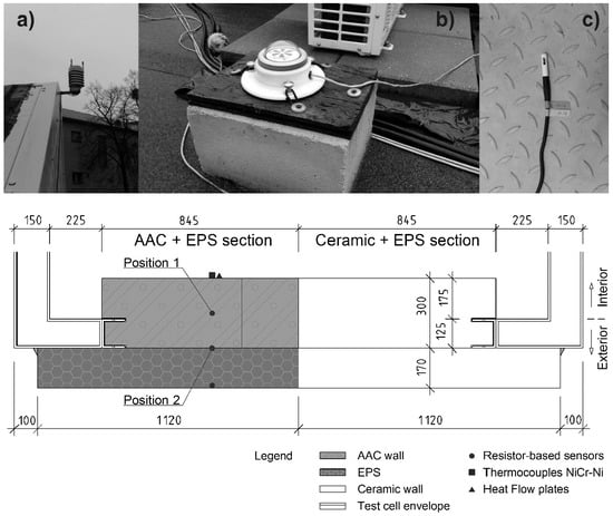
Figure 1.
Measuring equipment, instruments for measuring environmental values: (a) weather station; (b) pyranometer; and (c) temperature sensor and relative humidity of the air [28,29].

Figure 2.
Configuration of the wall of the test cell and the position of the measuring sensors. Section view of the AAC section [28,29].

Figure 3.
The measured outdoor air temperature in (°C) and the relative humidity of the air (%) for the locality of Košice. Displaying the selected period from May 2013 to December 2013 [28,29].

Figure 4.
Global Solar Radiation (W/m2). Measured data for the locality of Košice. Displaying the selected period from May 2013 to December 2013 [28,29].

Figure 5.
Sample structures, according to Table 2 (inside left). (a) An external test cell wall; and (b) simple AAC and sandstone walls. The placement position for the plotted data are: the calculated temperatures in Figure 8 and Figure 10 in specimen S2/S3, in Figure 12 and Figure 13 in S1 and the measured temperatures in Figure 15, Figure 16 and Figure 17 in specimen S1.

Figure 6.
Measured, sinusoidal and constant ambient air temperature over the selected time period as the boundary condition used to determine the initial temperature conditions, as according to Section 2.4.
Figure 6.
Measured, sinusoidal and constant ambient air temperature over the selected time period as the boundary condition used to determine the initial temperature conditions, as according to Section 2.4.

Figure 7.
The measured temperature values of the interior and exterior surfaces for the analyzed interval (14 February 2015 to 19 February 2015).
Figure 7.
The measured temperature values of the interior and exterior surfaces for the analyzed interval (14 February 2015 to 19 February 2015).

Figure 8.
Plotted temperature courses of the simple sandstone test wall S3 in Position 1, according to Table 2 and Figure 5b during the chosen time period.

Figure 9.
Temperature profile across the simple sandstone test wall at time t = 0 h, t = 12 h and t = 24 h for five cases under the initial condition. Abbreviations IC and BC refers to Section 2.4.
Figure 9.
Temperature profile across the simple sandstone test wall at time t = 0 h, t = 12 h and t = 24 h for five cases under the initial condition. Abbreviations IC and BC refers to Section 2.4.

Figure 10.
Plotted temperature courses of the simple AAC test wall S2 in Position 1, according to Table 2 and Figure 5b during the chosen time period.

Figure 11.
Temperature profile across the simple AAC test wall at time t = 0 h, t = 12 h and t = 24 h for five cases under the initial condition. Abbreviations IC and BC refers to Section 2.4.
Figure 11.
Temperature profile across the simple AAC test wall at time t = 0 h, t = 12 h and t = 24 h for five cases under the initial condition. Abbreviations IC and BC refers to Section 2.4.

Figure 12.
Plotted temperature courses of the outdoor test cell wall S1 in Position 1, according to Table 2 and Figure 5a during the chosen time period.

Figure 13.
Plotted temperature courses of the outdoor test cell wall S1 in Position 2, according to Table 2 and Figure 5a during the chosen time period.

Figure 14.
Temperature profile across the outdoor test cell wall (AAC + EPS) at time t = 0 h, t = 12 h and t = 24 h for five cases under the initial condition. Abbreviations IC and BC refers to Section 2.4.
Figure 14.
Temperature profile across the outdoor test cell wall (AAC + EPS) at time t = 0 h, t = 12 h and t = 24 h for five cases under the initial condition. Abbreviations IC and BC refers to Section 2.4.

Figure 15.
Plotted calculated and measured temperature courses in the outdoor test cell wall S1 in Position 1 during the chosen time period—with and without pre-calculation considerations.
Figure 15.
Plotted calculated and measured temperature courses in the outdoor test cell wall S1 in Position 1 during the chosen time period—with and without pre-calculation considerations.

Figure 16.
Plotted calculated and measured temperature courses in the outdoor test cell wall S1 in Position 2 during the chosen time period—with and without pre-calculation considerations.
Figure 16.
Plotted calculated and measured temperature courses in the outdoor test cell wall S1 in Position 2 during the chosen time period—with and without pre-calculation considerations.

Figure 17.
Temperature profile across the outdoor test cell wall S1 at t = 0 h, t = 24 h and t = 48—with and without pre-calculation considerations.
Figure 17.
Temperature profile across the outdoor test cell wall S1 at t = 0 h, t = 24 h and t = 48—with and without pre-calculation considerations.


Table 1.
Structure of the investigated perimeter wall (from the inside, the layers are in the direction of the heat flow) [28,29].
| No. | Test-Wall Layer | d (m) | λD (W/(m·K)) | c (J/(kg·K)) | ρ (kg/m3) |
|---|---|---|---|---|---|
| 1 | AAC | 0.300 | 0.104 | 900 | 350 |
| 2 | Foam PUR | 0.010 | 0.040 | 800 | 35 |
| 3 | EPS polystyrene graphite | 0.170 | 0.033 | 920 | 16 |
| 4 | Adhesive mortar | 0.002 | 0.850 | 900 | 1300 |
| 5 | Primer basic paint | - | - | - | - |
| 6 | Silicone additive plaster | 0.002 | 0.700 | 900 | 1700 |
Table 2.
Composition of the specimens (the layers are numbered from the inside in the direction of the heat flow) and physical properties of the material.
Table 2.
Composition of the specimens (the layers are numbered from the inside in the direction of the heat flow) and physical properties of the material.
| No. | Structure Specimens | Name of Layer | λ W/m·K | c J/kg·K | ρ kg/m3 |
|---|---|---|---|---|---|
| S1 | Outdoor test cell wall (AAC + EPS) | AAC | 0.106 | 900 | 350 |
| EPS | 0.035 | 920 | 16 | ||
| S2 | Simple AAC wall | AAC | 0.106 | 900 | 350 |
| S3 | Wall from sandstone | Sandstone | 1.700 | 840 | 2600 |
© 2019 by the authors. Licensee MDPI, Basel, Switzerland. This article is an open access article distributed under the terms and conditions of the Creative Commons Attribution (CC BY) license (http://creativecommons.org/licenses/by/4.0/).
Share and Cite
MDPI and ACS Style
Zozulák, M.; Vertaľ, M.; Katunský, D. The Influence of the Initial Condition in the Transient Thermal Field Simulation Inside a Wall. Buildings 2019, 9, 178. https://doi.org/10.3390/buildings9080178
AMA Style
Zozulák M, Vertaľ M, Katunský D. The Influence of the Initial Condition in the Transient Thermal Field Simulation Inside a Wall. Buildings. 2019; 9(8):178. https://doi.org/10.3390/buildings9080178
Chicago/Turabian StyleZozulák, Marek, Marián Vertaľ, and Dušan Katunský. 2019. "The Influence of the Initial Condition in the Transient Thermal Field Simulation Inside a Wall" Buildings 9, no. 8: 178. https://doi.org/10.3390/buildings9080178
Note that from the first issue of 2016, this journal uses article numbers instead of page numbers. See further details here.