

Modeling Firm Search and Innovation Trajectory Using Swarm Intelligence

1
Gabelli School of Business, Fordham University, 45 Columbus Avenue, New York, NY 10019, USA
2
Martin J. Whitman School of Management, Syracuse University, 721 University Avenue, Suite 500, Syracuse, NY 13244, USA
3
McCombs School of Business, University of Texas at Austin, 2110 Speedway, B6000, CBA 4.210, Austin, TX 78705, USA
*
Authors to whom correspondence should be addressed.
Algorithms 2023, 16(2), 72; https://doi.org/10.3390/a16020072
Submission received: 10 November 2022
/
Revised: 18 January 2023
/
Accepted: 19 January 2023
/
Published: 22 January 2023
(This article belongs to the Special Issue Applications of Evolutionary and Swarm Systems)
Abstract
:We developed a swarm intelligence-based model to study firm search across innovation topics. Firm search modeling has primarily been “firm-centric,” emphasizing the firm’s own prior performance. Fields interested in firm search behavior—strategic management, organization science, and economics—lack a suitable simulation model to incorporate a more robust set of influences, such as the influence of competitors. We developed a swarm intelligence-based simulation model to fill this gap. To demonstrate how to fit the model to real world data, we applied latent Dirichlet allocation to patent abstracts to derive a topic search space and then provide equations to calibrate the model’s parameters. We are the first to develop a swarm intelligence-based application to study firm search and innovation. The model and data methodology can be extended to address a number of questions related to firm search and competitive dynamics.
1. Introduction
Innovation is a major driver of firms’ financial performance and their ability to survive and adapt to changes in the business environment. Understanding firms’ search for innovations is therefore an important topic of inquiry. Prior research studied two broad antecedents to firm search—performance feedback [1] and competitive dynamics [2]. Although these antecedents have been studied using qualitative arguments and reduced-form empirical models, many of the most impactful insights into firm search have come from applying simulation models [3]. However, the field lacks a simulation tool that can incorporate competitors’ actions. This is an important gap because in many situations, the search activities of competitors will influence the firm’s own search strategy [4,5]. The current tools—the NK model and the multiarmed bandit—emphasize the firm’s own performance feedback but cannot model multi-agent interactions and are therefore, not well suited for this task. A complementary model is needed that can incorporate a range of competitive dynamics, and in this paper, we present such a model.
In this paper, we present a model to examine the technological “topics” a firm chooses to pursue. Our model is based on Reynolds’ classic Boids swarm program [6]. The model allows us to measure the firm’s position in the topic space and trace its path as it searches the space over time. The flexible model structure incorporates a variety of information that can influence what topics the firm searches, such as the firm’s own performance feedback and information on competitors’ positions and search trajectories.
We also demonstrate how to calibrate the model parameters using patent data. We take a novel approach to doing so, creating a topic space from patent data by using latent Dirichlet allocation topic modeling. The demonstration sample consists of 17 years of patent data and a sample of the firms in the information and communications technology industry (ICT) who most frequently patent in 11 of the United States Patent Office technology classes related to communication technologies. From the “test” sample, results show that the firms’ own performance feedback tends to predominantly inform their search trajectory. However, there is evidence that firms sometimes “flock” towards the same topic locations. Results also show that the large firms in our sample tend to differentiate from the leader rather than follow them. Note that these findings are simply demonstrative—we expect that a rich set of behaviors will play out in different samples and under different environmental conditions.
The paper is structured as follows. Section 2 briefly reviews the related literature. Section 3 describes the model framework and data. Section 4 provides some examples of how to fit the model to a topic landscape defined by patent data and provides some example results. Section 5 compares our swarm model to the NK and multiarmed bandit models. Section 6 provides a discussion of our model and directions for future research. Section 7 concludes. Appendix A provides an appendix with the swarm pseudocode.
2. Background
Research on firm search traces its roots back to the early literature on the behavioral theory of the firm [7]. Unlike neoclassical economics that tends to treat decision makers as hyperrational with the ability to search over all possible solutions, the behavioral theory of the firm postulates that managers have imperfect information and are boundenly rational, thus willing to make satisfactory rather than optimal decisions [8]. Therefore, when faced with a problem, firms typically conduct a “local search”—searching for solutions within the neighborhood of their current knowledge. Building on these concepts, classic work in evolutionary economics suggests that the firm’s search process will lead it to be “path-dependent” [9]—i.e., the technological topics the firm searches today will influence what technological problems it will search and solve in the future [10,11]. (Note that we incorporate the possibility of path dependence in our model).
Much of the recent search-related literature on innovation and technology strategy has focused on four questions related to firm search. First, what strategies can firms use to overcome path dependence and perform distant search effectively [12,13,14,15,16,17,18]? Second, how can firms effectively balance exploration of new and exploitation of current knowledge and capabilities [19,20,21,22,23,24]? Third, what can be learned about search by studying individuals or teams [25,26,27,28,29,30]? Fourth, how does competition shape search strategies [31,32,33,34,35]? While prior research has studied all of these questions using qualitative arguments and reduced-form empirical models, simulation tools have only been applied to the first three.
Scholars examining firm search and innovation trajectories have long relied on simulation models to illuminate new insights [3] For instance, scholars like Nobel Prize and Turing winner Herbert Simon, whose work on the decision-making processes within firms formed the early foundation of the behavioral theory of the firm, suggested that simulation models were useful tools for studying firm search and decision problems and he helped pioneer the development and application of such models in his analysis of problem-solving behavior in organizations [36]. Since then, many of the most influential papers on firm search and learning have used simulations (e.g., March (1991)) [37].
The most popular model used to study search and organizational learning is the NK model, originally developed by biologist Stuart Kauffman [38]. The NK model uses two parameters to create a potentially rugged fitness or performance landscape—with N capturing the number of elements in the landscape and K capturing the extent to which the elements are interdependent. The points on the landscape represent a combination of choices among the N elements and the height of the landscape at a particular point represents performance. The performance contribution of each component (ci) depends on K other interdependent components. Therefore, the performance of a position on the NK landscape is determined by the sum of the component-level performance contributions for that position. This value is typically normalized by dividing it by N so that performance can be compared across landscapes with different values for N. The smoothest landscape occurs when K = 0, where all components are independent and only one optimum is defined. As K increases, the landscape becomes more peaked and rugged, with peaks varying in height, creating multiple local optima. The landscape is most rugged when K = N − 1, i.e., all components are dependent on all other components. At a peak, changing the value of one component will not improve performance, instead, the values of multiple components must change for performance to improve. See Csaszar (2018) for more technical details about NK landscapes [39].
The NK performance landscape can be used to represent a variety of complex organizational problems that have a performance landscape that the simulated managers can “search.” The more rugged the landscape (higher K), the more challenging the search process and the greater chance that simple sequential search strategies will result in low performance [40]. For instance, a simple search strategy in which the manager changes one component at a time is unlikely to effectively identify a global optimum in a rugged landscape.
Prior research has applied NK to a number of business problems in which the firm must search for a solution among many interdependent elements. For instance, researchers have used NK to examine adaptation to a changing external environment [41,42], the influence of organizational design on search [43,44], coordination within a multi-business firm [45], and innovative search within ecosystems [46].
Although the NK model has proven to be a powerful tool, it has several limitations when applied to the study of a firm’s search for innovations. First, the NK model focuses on search on the performance landscape without incorporating any other influences. Therefore, the model has a firm-centric focus. Second, the ability to incorporate information from the environment is limited. For instance, Levinthal (1997) incorporated environmental change into the NK model through a reorientation of the entire landscape. There does not appear to be an easy way to incorporate multiple sets of competitor actions or complex external dynamics into the model.
Another useful (but less used) formulation to study firm search behavior is the multiarmed bandit model. The literature on economics, strategy, and computer science uses the multiarmed bandit model to represent exploration–exploitation problems. The model allows for the study of how managers allocate resources or make search decisions under payoff uncertainty [47]. For example, Posen and Levinthal (2012) used the multiarmed bandit model to examine exploration and exploitation in response to environment change. Like the NK model, it is difficult to incorporate non-firm centric information in a rich way. In Posen and Levinthal’s study, they only incorporated environmental information as a stochastic shock to the payoff values. Overall, NK and Bandit models do not appear to be easily extended to incorporate the search behaviors of other actors, thereby prompting the need for a different approach.
Swarm intelligence offers another approach to dynamic search problems. Inspired by the natural world [48], swarm intelligence systems use a population of independent agents that can be made to interact with their environment and with each other [49,50]. Swarm intelligence has found a wide set of applications in the physical and social sciences. One of the most fruitful areas of application has been the study of optimization problems [51,52]. Particle swarm optimization (PSO) moves ‘particles’ around a search space to discover the best position (global optimum) [53]. In the standard PSO, particles are guided by simple formulas that define their velocities and update their positions in the search space. PSO algorithms have been improved and extended to increase their speed, accuracy, and ability to tackle more difficult optimization problems [54,55,56,57]. See Sengupta, Basak, and Peters (2018) for a survey of the PSO literature [58].
Prior literature in business and economics has used swarm intelligence, particularly PSO, to solve business-related optimization problems. For instance, in the field of financial economics, particle swarm has been used for portfolio optimization [59], efficient frontier estimation [60], interest rate modeling [61], and earnings forecasting [62]. Within the strategy and organization literature, Coen and Maritan (2011) used a version of swarm to study resource allocation under uncertainty [63]. Utilizing the SWARM software of Minar, Burkhart, and Langton (1996), they developed an agent-based model of resource allocation, exploring how the firm’s search ability and initial capability endowment influence performance in a competitive environment.
3. Materials & Methods
In this section, we derive a framework that can incorporate a wide range of information—behaviors of competitors, the firm’s performance on its own fitness landscape, etc.—that can influence what technological topics the firm will search. We take our inspiration from Reynolds’ (1987) model of swarm behavior of animals such as bees, fish, and birds because how firms move within a landscape has similarities to the well understood swarm behavior of these animals. In his Boids model of swarm or flocking behavior, Reynolds (1987) formulated the algorithm from three key parameters: cohesion, alignment, and separation. By various combinations of these parameters, one can specify a desired behavior for the flock of birds or a school of fish. We extend this model to the study of firm search behavior. In Section 3.1, we present the basic modeling framework that can be used to run a simulation. In Section 3.2, we introduce a novel approach to deriving a topic space from patent data as well as describe the data that we use to fit the model.
3.1. Model Development
Let there be firms and technological topics (henceforth called topics). At each given point in time t, we map firm i’s location in the topic space. The resulting map forms an n-dimensional hypercube image of the topics, with each axis of the hypercube representing each jth topic. Comparing the firm’s location across time (e.g., t to t + 1) allows us to represent its migration within the topic space.
In this version of the model, we bounded each axis as continuous variable between 0 and 1 (other lengths could be chosen without loss of generality). Therefore, the firm’s location on that axis can be thought of as the propensity for the firms’ innovations at time t to relate to topic j. If a firm has more than one innovation at time t, where the firm lies in [0,1] on axis j will depend on the average across the innovations. For instance, if five innovations focus on topic j (=1) and five do not (=0), then the value for j = 0.5. We discuss how we handle real world patent data in Section 3.2.
We defined firm i’s position at time t using the vector of topics, where is the jth element. For the sake of completeness, we defined as the set of firms whose positions at time we defined by the matrix .
We defined the velocity of a firm as follows:
where the weights () sum to 1. A, C, and S stand for alignment, cohesion, and separation, respectively, which we derived from Reynolds’ (1987) swarm program. L and P stand for leader following and performance feedback, which we describe below. We defined these three velocity vectors as follows:
Alignment determines the firm’s propensity to move (or in our case, search) in the direction of a competitive reference group. When the weight on alignment is high, firms will shift the direction of their search as the firms within the reference group change their search direction. A set of firms with high alignment will appear to ‘flock’ together, or in our applied case, searching the same technologies. When the weight is low, shifts in the reference group’s behavior have little influence on the focal firm.
Cohesion determines the firm’s propensity to move towards the average position or center of mass of its competitors. When modeling animal behavior, such as a flock of birds, cohesion controls how tightly they stay together. In firm search, when a firm has high cohesion, it searches closer to the search positions of its reference group.
For both alignment and cohesion, the reference groups (F) can be defined flexibly so as to encompass the competing firms that most likely influence the focal firm’s search. Therefore, Equations (2) and (3) can be used to model a wide range of competitive imitation strategies.
Separation determines whether firms can take the same position as other firms within the hypercube. The ε parameter in (4) can be thought of as the minimum separation threshold between firms on the search space. Setting ε = 0 allows for collocation, while setting ε to a very small number insures some minimal “separation”.
In addition to the three classic parameters—alignment, cohesion, and separation—we added two additional ones that capture theoretically interesting firm search behavior. Evolutionary economic models suggest that firms will be influenced by their past performance and may exhibit path-dependent behavior. To incorporate this element into our model, we defined the following equation:
where, for the th firm, is a uniform random number in [0,1], is the historical personal best (measured by the fitness function), and is a weight allowing the firm to choose between full exploration (which is a totally random move) and full exploitation (only follow its own personal best).
Organizational theory suggests that a firm may follow specific competitors, such as the leader in the market [64]. We modeled this possibility as follows:
where is the leader’s position which is chosen from all the personal bests and is a scaler to gauge how a firm decides to follow the industry leader, e.g., a negative indicates that the firm chooses to move away from the leader. In our demonstration, we defined the leader based on who has the highest performance at time t − 1. The ability to define in a variety of ways allows for a simple yet flexible way of modeling a variety of variations of imitative behavior.
To update a firm’s position, we used the following formula:
In Section 4, we describe how to fit this model to data and provide some example results on a test sample of patent data.
In a simulation of firms’ behaviors, one starts with a randomly chosen landscape (-dimensional ) with a set of chosen parameter values , and . These allow one to first calculate Equation (2) through (6) and then Equation (1). Once the velocity (Equation (1)) is calculated, the next landscape can be calculated by Equation (7). The process repeats as many times as one desires. In a long simulation, the parameters that describe the initial landscape are ultimately irrelevant. For example, if , , and are high, then the swarm will converge to a single point ultimately. Or alternatively, if and are high, then firms move in a group (much like a school of fish).
Note that while the parameter values could change over time, they are not made to do so. This is because we want to observe the search behavior over time (e.g., so that we can examine if firms converge or diverge from each other). Most likely, in real situations such as ours they will be time-varying. However, an empirical concern is whether there is enough data to solve for time-varying parameters. This issue is discussed in the next section.
In our empirical work here, we used data to solve for the parameter values in order to examine and explain how firms interact with one another. Using data, we first obtained all the positions of all the firms, i.e., for all . This allowed us to calculate all the (empirical) velocities by taking the difference of two consecutive landscapes using Equation (7). In the broadest sense, all the parameters can be solved at once. However, this might result in a situation in which parameters become uninterpretable. We hence chose to study the two most relevant velocities (behaviors) in our data—leader following (Equation (6)) and firm exploration (Equation (5)). Then we combined these partial results into a grand optimization. Details are explained in the next section.
In solving the parameters, we discovered that in some cases, closed form solutions (of the parameters) can be derived. This can be easily done via taking derivatives of the fitness function with respect to the parameters. Details are given in the next section.
A pseudo code is provided for a more clear description of the algorithm in the Appendix A, swarm(w_a, w_c, w_l, w_p, ntim). In a simulation, the values of these swarm parameters are pre-determined. The swarm algorithm computes the fitness value, personal best, and the global best in each iteration. Then the entire history of movements of the particles (firms) are recorded and studied. In this paper, fitness value, personal best, and global best (along with firm positions in topic space) are input from data. We then set ntim=1 and solve for the four parameters in each iteration.
3.2. Data
To examine a firm’s innovative search direction, we need information on its R&D projects. While this information is not typically publicly available, we can assess the outcomes of their successful searches by using patent data. Patent data has been a key source of information on innovation in the strategy and economics literature [65].
Data on U.S. patents and patent citations come from the U.S. Patent and Trademark Office (USPTO) and the Patent Network Dataverse [66], for which firm-level identifiers have been mapped in prior research [67,68]. For each patent, we used the abstract, assigned technology class, patent assignee, and the patent’s application date. To tie a patent to a year (our unit of time in our study), we used application dates rather than grant dates because the application date better approximates the time in which the firm searched the topic.
In our demonstration, we used patent data on the 11 3-digit USPTO patent classes most closely associated with communications technologies (see Table 1) during the period 1985–2007. The sample timeframe and patent classes have been used extensively in the prior technology strategy and innovation economics literature, e.g., [69,70]. We selected communication technologies for several other reasons. First, firms in this industry tend to patent most innovations. Therefore, patent data likely reflect the search behavior of these firms. Second, the time between the initial outlays for R&D and patenting is short compared to other areas like drug discovery, thus using the firm’s patent application dates is a good proxy for its current search focus. Third, prior work on this industry suggests that firms might exhibit a variety of search behaviors.
Much of the prior innovation literature in strategy and economics uses the 3-digit technology class or the lower level, subclass, to categorize patents [71]. However, using such levels of classification schemes, while useful in many research settings, may not be sufficiently nuanced for our purposes. For instance, firms searching for innovations within multiplex communications (technology class 370) may focus on a variety of topics (space division multiplexing, code division multiplexing, time division multiplexing, etc.). To best perform the analysis, a more nuanced measure of “topics” is needed.
We used latent Dirichlet allocation (LDA) to create topics from patent abstracts. LDA is a commonly used, unsupervised machine learning technique to create topics from text [72]. Most work on LDA uses the researchers’ own inputs to define the number of topics, however, that can be problematic in this setting for two reasons. One, researchers may not have the expertise to suggest the appropriate number of topics within a technology class. Two, creating an algorithm to select topic size may allow for more consistency across researchers and remove the potential of user-induced measurement bias. Therefore, we chose the number of topics by maximizing the coherence score, a commonly used construct in LDA that measures how similar the words on a topic are to each other. In this sample, we used the CV coherence score [73] to choose topics. Several other commonly used alternatives—UMass coherence Score, UCI coherence Score, and Word2vec coherence score—produce similar results.
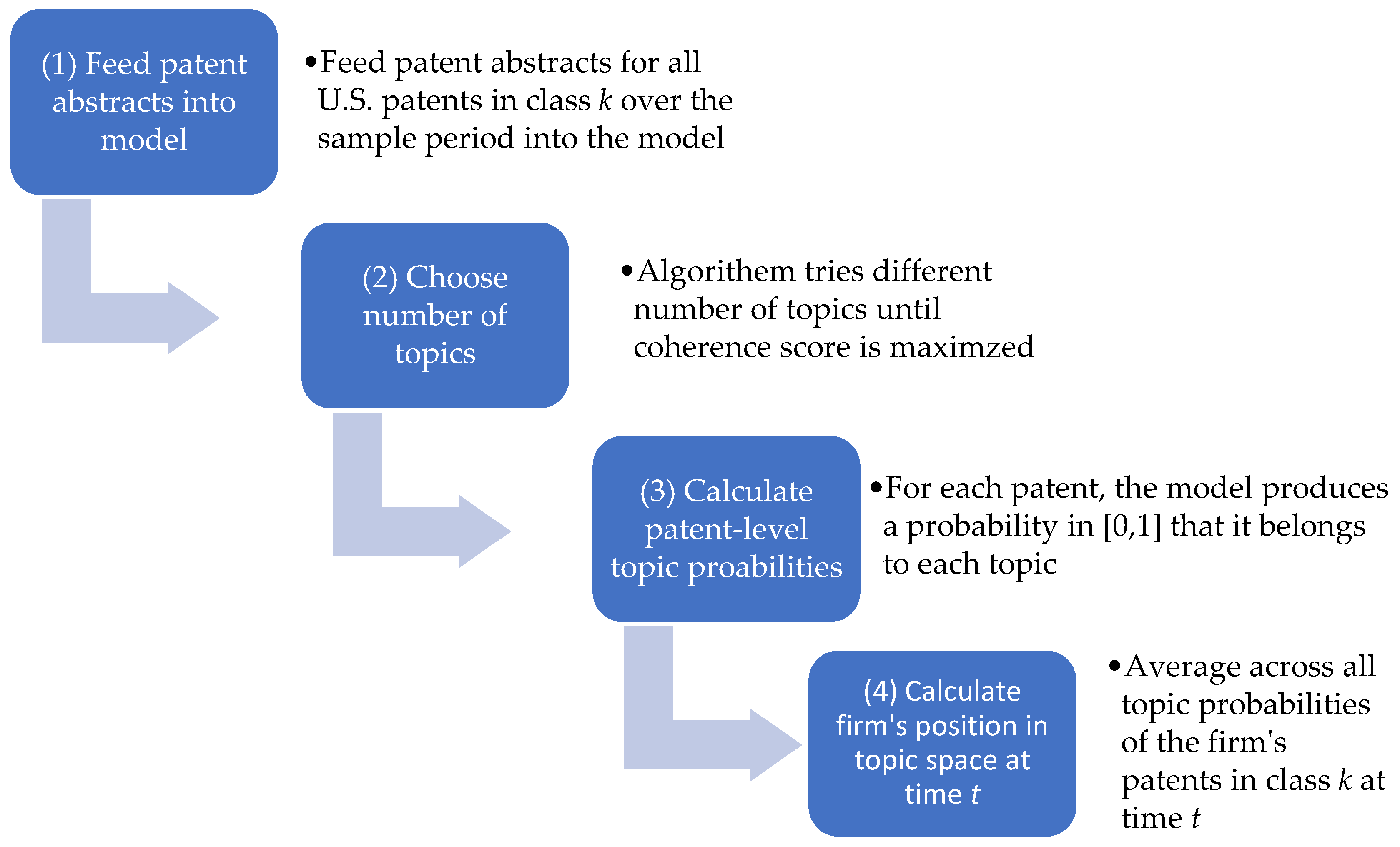
To create the topic space, for each patent class, we fed all patent abstracts for the entire sample period in to the LDA model using the LDA program from the Natural Language Toolkit in Python. Note that all U.S. patents during the entire sample period were used, not just patents from the firms that we studied. The number of topics that maximizes the coherence score was chosen, which determines the n-dimensional hypercube. LDA provides a probability that each patent is associated with a particular topic. For each firm in each year t, the coordinate in the cube (e.g., position on each axis j) is calculated by averaging the probabilities across all the firm’s patents. We summarize the process for obtaining a firm’s position in topic space from patent data in Figure 1.
To create a tractable sample of firms for demonstration purposes, we included only public firms that were in the top 20 in terms of patenting in each of the 11 technology classes. This yielded a total of 32 large firms that are extremely active in the communication technologies space. Note that such a sample should bias our model findings away from follow-the-leader and imitative strategies, as these firms are the leaders who will most likely follow their own feedback.
The resulting sample has 11 separate topic landscapes (one for each technology class). The number of topics varies from 10 to 47 depending on the technology class. The time dimension (t) was set to a year, and we calibrated the parameters using the 1991–2007 period. Note that we started our analysis in 1991 when communication technology patenting had more density.
4. Results
In this section, we discuss how to fit our model to actual data in order to calibrate the parameters. We start by illustrating how to fit a partial model that captures specific behavior—in this case, the firm following its own performance feedback and following the leader. We then fit the entire model.
Firm’s personal best (path dependency)
We begin by only allowing for the firm’s own feedback to guide its innovation trajectory. In Equation (1) we set and all other weights to 0. Equation (1) then converges to Equation (5) only. We should note, that in theory there is no limitation on the value of velocity, yet in our empirical work, the velocity is confined to be the difference between two consecutive landscapes.
We define data-based (empirical) positions as and calculate velocity as follows:
Our objective function is to minimize the sum of squared errors between and :
We then solve the coefficient analytically as:
where
is the personal best and is the fitness (performance) function.
To calculate fitness or performance for firm i, we need some measure of firm performance that can be directly tied to its position in the topic landscape. We use a patent-based measure of performance—forward citations. Forward citations—citations from other patents the focal patent receives—have been shown to be a good proxy for financial value of an innovation and are commonly used as a measure in the economics and strategic management literature [74]. To calculate performance, we take the average number of forward citations across all the successfully granted patents that the firm applied for in the technology class in year t. We provide descriptive statistics to summarize results (across firms and across time) for each technology class in Table 2.
Results in Table 2 indicate that firms closely follow their own feedback, with very close to 1. Note that this result is similar to a partial derivative with respect to the personal best. That is, holding other behavioral patterns constant, firms always “remember” their best performing locations in topic space.
Following The Leader
We demonstrate two simple ways to model leader-following behavior.
where in the former each firm has its own leaders () and in the latter all firms share the same leader (). The objective is slightly modified as :
The solution is
The results are summarized in Table 3 (where all firms have the same leader in each year), Table 4 (where each firm has a different leader), and Table 5 (which provides further descriptive statistics for when each firm has a different leader).
Table 3 indicates that firms do not follow an industry leader (with all exhibiting negative values), rather, firms tend to move away from or “differentiate” from the leader. We observe some variations among different classes and different years. Firms in technology classes 370, 375, 379, and 398 exhibit greater tendency to move away from their industry leaders than in other classes. From the mid-1990s to the early 2000s, tendencies to move away from industry leaders were stronger than in other years.
is different for each firm. The above table summarizes all firms over all years.
Table 4 tells a similar story to Table 3, yet the magnitudes are stronger. In Table 4, we allow each firm to have a different coefficient toward its leader. Then we take an average across all firms in the same class/year. The results are now at several times of those in Table 4. Properties of the distribution are provided in the next table (Table 5).
A distribution is provided in Table 5 by patent class. Table 5 sheds some light on the details of . While averages (Table 4) are all negative, Table 5 indicates that a certain percentage within each class still is positive. Take 340 as an example, nearly 40% of firms in this class have a positive .
Full Model
In this section, we calibrate the full model. Because firms can take the same position in topic space—e.g., firms can search for similar innovations—we can omit the separation equation, and hence set . We let the other four forces that drive the swarm remain. Without loss of generality, we can set to simplify the problem. In sum, we will solve for , , , , and in the simultaneous equation system. The pseudo code of the estimation is given in Figure 2 below:
Note that in the above pseudo code, the positions (i.e., topics) are input and velocities are calculated off consecutive positions. The personal best (pbst), and global best (gbst) are also input. In a simulation, ntim (number of iterations) is set and all movements are recorded (including the fitness value). In our study, since we already have all of the positions, we solve for the parameters w_a, w_c, w_l, w_p by reading in the personal best and global best, and setting ntim=1.
As mentioned earlier (Section 3.1), the weights that determine the velocity (see Equation (1)) are generally fixed over time because the objective is to observe how the swarm behaves in the long run. However, in our case, we have data on firm behavior each year, hence, our interest is to examine if the observed behavior varies over time. In other words, do the parameters change as the firms respond to changes in their environment. We show the yearly weights across the four parameters in Table 6. The results indicate that the firm’s own personal best and to a lesser extent, alignment, influence search behavior the most. The other two factors, cohesion and following the leader, receive minimal weight in most years.
5. Model Comparison
The proposed swarm-based search model differs from the two complementary models (i.e., NK and multiarmed bandit) in multiple ways. First, the best application differs across the models. NK is ideally suited to examine complexity, which is a useful way to represent knowledge recombination or the interdependencies between elements in an organizational design problem. Researchers use multiarmed bandit models to model the exploration–exploitation problem. Neither of these models ideally fits the objective of modeling a firm’s search across innovation topics.
Second, the models differ in how they utilize performance feedback. In NK, the N and K parameters create a potentially rugged performance or fitness landscape that provides information to the firm as it searches. The multiarmed bandit model reveals information on payoffs as the agent makes commitments to search a particular dimension (e.g., pulls a particular lever). In our current version of the swarm search model, feedback is defined by empirically estimated performance based on observed outcomes. The firm’s best performance is allowed to influence the direction of search. The NK and multiarmed bandit allow for more complex feedback; for instance, the agent searching a landscape may be allowed to view performance of other locations.
Third, the models differ in how the general environment and the action of competitors (or other agents) influence search behavior. Neither NK nor bandit models are optimized for competitive dynamics. Environmental change typically comes into these models in a simple way, by exogenously shocking payoffs. The swarm search model can capture a richer set of competitive behaviors.
Overall, these models appear optimized for different tasks and therefore are complementary. Table 7 summarizes the key differences in these models as applied to firm search.
To understand the differences in application, compare this paper with a study by Ganco (2017) [75], which uses the NK model to generate predictions regarding the performance–knowledge recombination relationship and then tests these predictions empirically using patent data in US Patent Class 360. Specifically, Ganco (2017) models forward citations of patents (a measure of patent performance) as a function of N (empirically measured as the number of patent subclasses cited by the focal patent) and K (interdependence of the subclasses inferred from prior patents’ recombination of subclasses). The results suggest that performance of a patent has an inverse U-shaped relationship with the complexity of the knowledge being recombined. Note that the focus of Ganco (2017) is on how the performance of an innovation is affected by the way in which the focal firm recombines prior knowledge. This focus differs from ours—we focus on the factors that influence what technologies the firm will search.
6. Discussion
In the current model specification, we allow for firms to follow their own feedback (), follow the leader (), move to the current location of their competitors (cohesion, ), or move in the direction of where competitors are headed (alignment, ). We also define separation per the original Boids program (). Below we discuss each of these factors and how they might be augmented for future research.
Firm Feedback/Path Dependency
We take a simple approach to modeling the firm’s own feedback, using only a parameter that captures of how the firm’s best performing location influences its movement through topic space. Anchoring on best performance has a parallel in the literature on NK modeling where the firm searches for the highest peak on the performance landscape. Future work could embellish this equation to capture the complexities of how the firm’s own search history influences its future search behavior. For instance, the firm’s prior search trajectory (rather than its best performance), represented by prior (lagged) positions in search space, could be included to model search inertia. In addition, variables that capture prior changes in performance on the performance landscape (e.g., lagged values along the gradient) could be added to incorporate more complex information on performance feedback into the model. Uncertainty, like in the bandit model, could be added by including feedback noise.
Follow The Leader
We offer two simple approaches to modeling leader-following behavior. Firms can follow a global leader or a local leader, defined by a function or the firm’s choosing. By modifying how to specify the leader(s), future work can fit the model to a wide range of behaviors proposed by strategy management and organizational theory literature. Competing theories on imitation, differentiation, and the general influence of a firm’s peers can be tested or simulated using this framework.
Note that leader-following behavior does not appear to be prominent in our demonstration sample. This is not surprising given that these are the ‘leading’ firms in terms of patenting during out sample period. However, smaller firms and less technologically sophisticated firms may display a range of interesting behaviors. Prior literature suggests that such firms may follow cues of the leaders, which would appear as following the leader in our model. Other work suggests that firms might steer away from more technologically sophisticated leaders. Future work could use our model to shed light on these behaviors.
Cohesion
In a typical swarm model of animal behavior, cohesion represents how closely the focal actor stays to the center mass of the group. By adjusting cohesion, more concentrated (higher cohesion) or more diffuse (lower cohesion) swarming behaviors can be simulated. Applied to firm search, the current specification for cohesion represents the extent to which firms cluster in similar areas in topic space. To simulate a wide range of imitative behavior proposed in the sociology, organizational theory, or strategy literature, this equation can be adjusted by changing the set of firms in the reference group. The cohesion equation can also be extended to incorporate other information, such as multiple reference groups or performance-weighted reference groups, which can allow the research to closely map extant theories.
Alignment
In a typical swarm model of bird behavior, alignment represents how agents move towards the heading of their reference agents. We use this specification of alignment to examine how firms adjust their search towards the direction their reference group is heading. By including information of competitors’ “direction” we can study how the expected search behavior of competitors influences the focal firm. As with cohesion, by adjusting the reference group, we can study a wide range of behaviors of interest to strategy and organizational theory scholars.
Separation
Separation plays a role in the typical artificial life programs by keeping the agent from colliding with other agents—e.g., birds do not typically run into other birds in the same flock. In our model, there is no reason why firms cannot search the same “topics.” Thus, we omit separation for theoretical and computational simplicity. However, separation could play a useful role in innovation simulations. For instance, if the “space” was altered to be unique patents rather than innovation topics, then firm k’s position in such space might prohibit firm i’s ability to legally assume the same location (e.g., a patent provides the owner the ability to attempt to preclude another from copying the innovation). When studying such cases, separation could be a theoretically interesting addition to the modeling framework.
Caution In Interpreting Model Parameters
We urge caution in interpreting the estimated parameters of the models as causal. For instance, the theorical foundation for following the leader, alignment, and cohesion is that the firm imitates others. However, separating “imitation” from the firm’s response to similar environmental cues (often called ecological effects) or because they have similar individual characteristics (often called correlated effects) is exceptionally difficult [76]. Identification can be obscured by the fact that the researcher cannot tell if the firm is responding to the action of competitors, or instead responding to the same latent environmental factors as all other firms in the reference group or if all firms in the reference group have similar latent properties that cause them to search in a similar manner as the focal firm.
7. Conclusions
Simulation models have been successfully applied to the study of firm search. Leading simulation models, like the NK model and the multiarmed bandit, have illuminated how the firm’s own performance feedback influences search, but these models ignore the influence of competitors. This is particularly problematic in settings in which competitive dynamics may play an important role. To address this need, we developed a model based on the Boids algorithm, which we applied to the study of firms’ search for innovations. The model can incorporate a rich set of information on competitor behavior, as well as information on the firm’s own performance. We demonstrate how to fit the model to patent data and offer a novel approach to developing a “topic space” applying LDA to patent abstracts.
Results from fitting the model to the test data show that either performance feedback or alignment with competitors tend to drive firms’ search trajectories. Consistent with prior literature, firms take cues from their past search performance. At times, firms also flock together (high alignment), which may suggest that there is a competitive influence or rather, that all firms are responding to the same environmental cues. We expect a combination of both in this sample. Future research can develop ways to tease apart competitive influence from ecological effects.
The results based on this test data do not support leader-following behavior, though this is not surprising given that the firms in our sample are large “industry leaders,” and likely differentiated to some extent. Future research can apply the model to different contexts and different types of firms.
We make two contributions to the literature on firm search. First, leading simulation models do not incorporate competitor behavior into their models, which has limited the field’s ability to use simulations to address questions in which competitive dynamics are salient. The model posed here addresses this issue and provides the field a tool to complement the NK and bandit models. Future research can apply this model to examine a wide range of search questions.
Second, our approach to creating topic landscapes from patent data using LDA has promising applications not only in the study search, but in other areas of the strategy and innovation literatures in which patents are typically used. Our process allows researchers to uncover more nuanced similarities between patents than what can be done using the USPTO patent classification system or by drawing inference based only on the commonly used characteristics of the patents (e.g., backwards citations). The more nuanced measures of topics can help scholars to better measure commonly used constructs like knowledge relatedness.
As a final thought, it is worth noting that swarm intelligence models and evolutionary-based algorithms developed for natural science, computer science, and engineering applications may have useful applications in the strategy and managerial science literature. For instance, PSO applications have developed rapidly in the past decade, and many could have useful applications to strategy problems like search modeling. We refer you to the recent PSO references in Section 2 (e.g., Zhan et al., 2008; Michaloglu and Tsitas, 2021) as starting point for further inquiry.
Author Contributions
Conceptualization, C.D.M., R.-R.C. and P.K.T.; Methodology, C.D.M. and R.-R.C.; Programming, R.-R.C.; Validation, R.-R.C.; Formal Analysis, C.D.M. and R.-R.C.; Data Curation, C.D.M.; Writing—Original Draft Preparation, C.D.M.; Writing—Review & Editing, C.D.M., R.-R.C. and P.K.T. All authors have read and agreed to the published version of the manuscript.
Funding
This research received no external funding.
Data Availability Statement
Data can be accessed from the United States Patent and Trademark Office or from Harvard Dataverse—Patent Network Dataverse (https://dataverse.harvard.edu/dataset.xhtml?persistentId=doi:10.7910/DVN/5F1RRI (accessed on 9 November 2022)).
Acknowledgments
We thank Eugene Pyun of Fordham University for his assistance with LDA topic modeling.
Conflicts of Interest
The authors declare no conflict of interest.
Appendix A
Figure A1 provides the full pseudo code for the program.
Figure A1.
Swarm Pseudo Code.

Note: The fitness function fcn_obj computes the fitness value. In our study, fitness values are an input. Additional inputs are personal best pbst and global best gbst. In a simulation, ntim (number of iterations) is set and all movements are recorded (including the fitness value). In our study, since we already have all the positions, we solve for parameters w_a, w_c, w_l, w_p by reading in the fitness value, personal best, global best, and set best, and set ntim=1.
References
- Levinthal, D.A. Adaptation on Rugged Landscapes. Manag. Sci. 1997, 43, 934–950. [Google Scholar] [CrossRef]
- Katila, R.; Chen, E.L. Effects of Search Timing on Innovation: The Value of Not Being in Sync with Rivals. Adm. Sci. Q. 2008, 53, 593–625. [Google Scholar] [CrossRef] [Green Version]
- Levinthal, D.A.; Marengo, L. Simulation modelling and business strategy research. In The Palgrave Encyclopedia of Strategic Management (1–5); Palgrave Macmillan: London, UK, 2018. [Google Scholar]
- Lieberman, M.B.; Asaba, S. Why do firms imitate each other? Acad. Manag. Rev. 2006, 31, 366–385. [Google Scholar] [CrossRef] [Green Version]
- Clarkson, G.; Toh, P.K. ‘Keep out’ signs: The role of deterrence in the competition for resources. Strateg. Manag. J. 2010, 31, 1202–1225. [Google Scholar] [CrossRef]
- Reynolds, C. Flocks, herds and schools: A distributed behavioral model. In SIGGRAPH’87: Proceedings of the 14th Annual Conference on Computer Graphics and Interactive Techniques; Association for Computing Machinery: New York, NY, USA, 1987; pp. 25–34. [Google Scholar]
- Augier, M.; Prietula, M. Historical roots of the ‘a behavioral theory of the firm’ model at GSIA. Organ. Sci. 2007, 18, 337–545. [Google Scholar] [CrossRef]
- Cyert, R.; March, J.G. A Behavioral Theory of the Firm; Blackwell Business, Ltd.: Oxford, UK, 1963. [Google Scholar]
- Nelson, R.R.; Winter, S.G. An Evolutionary Theory of Economic Change; Belknap Press: Cambridge, UK, 1982. [Google Scholar]
- Siggelkow, N.; Levinthal, D. Escaping real (non-benign) competency traps: Linking the dynamics of organizational structure to the dynamics of search. Strateg. Organ. 2005, 3, 85–115. [Google Scholar] [CrossRef]
- Gavetti, G.; Levinthal, D. Looking Forward and Looking Backward: Cognitive and Experiential Search. Adm. Sci. Q. 2000, 45, 113–137. [Google Scholar] [CrossRef] [Green Version]
- Ahuja, G.; Lampert, C.M. Entrepreneurship in the large corporation: A longitudinal study of how established firms create breakthrough inventions. Strateg. Manag. J. 2001, 22, 521–543. [Google Scholar] [CrossRef]
- Rosenkopf, L.; Nerkar, A. Beyond local search: Boundary-spanning, exploration, and impact in the optical disk industry. Strateg. Manag. J. 2001, 22, 287–306. [Google Scholar] [CrossRef]
- Fleming, L.; Sorenson, O. Science as a map in technological search. Strateg. Manag. J. 2004, 25, 909–928. [Google Scholar] [CrossRef]
- Laursen, K. Keep searching and you’ll find: What do we know about variety creation through firms’ search activities for innovation? Ind. Corp. Chang. 2012, 21, 1181–1220. [Google Scholar] [CrossRef]
- Mudambi, R.; Swift, T. Knowing when to leap: Transitioning between exploitative and explorative R&D. Strateg. Manag. J. 2014, 35, 126–145. [Google Scholar] [CrossRef]
- Eggers, J.P.; Kaul, A. Motivation and Ability? A Behavioral Perspective on the Pursuit of Radical Invention in Multi-Technology Incumbents. Acad. Manag. J. 2018, 61, 67–93. [Google Scholar] [CrossRef] [Green Version]
- Randle, D.K.; Pisano, G.P. The Evolutionary Nature of Breakthrough Innovation: An Empirical Investigation of Firm Search Strategies. Strateg. Sci. 2021, 6, 290–304. [Google Scholar] [CrossRef]
- He, Z.-L.; Wong, P.-K. Exploration vs. Exploitation: An Empirical Test of the Ambidexterity Hypothesis. Organ. Sci. 2004, 15, 481–494. [Google Scholar] [CrossRef]
- Andriopoulos, C.; Lewis, M.W. Exploitation-Exploration Tensions and Organizational Ambidexterity: Managing Paradoxes of Innovation. Organ. Sci. 2009, 20, 696–717. [Google Scholar] [CrossRef] [Green Version]
- Hoang, H.; Rotheraermel, F.T. Leveraging internal and external experience: Exploration, exploitation, and R&D project performance. Strateg. Manag. J. 2010, 31, 734–758. [Google Scholar]
- Fang, C.; Lee, J.; Schilling, M.A. Balancing Exploration and Exploitation Through Structural Design: The Isolation of Subgroups and Organizational Learning. Organ. Sci. 2014, 21, 625–642. [Google Scholar] [CrossRef]
- Fitzgerald, T.; Balsmeier, B.; Fleming, L.; Manso, G. Innovation Search Strategy and Predictable Returns. Manag. Sci. 2021, 67, 1109–1137. [Google Scholar] [CrossRef]
- Stagni, R.M.; Fosfuri, A.; Santaló, J. A bird in the hand is worth two in the bush: Technology search strategies and competition due to import penetration. Strateg. Manag. J. 2021, 42, 1516–1544. [Google Scholar] [CrossRef]
- Fleming, L.; Mingo, S.; Chen, D. Collaborative brokerage, generative creativity, and creative success. Adm. Sci. Q. 2007, 52, 443–475. [Google Scholar] [CrossRef] [Green Version]
- Gruber, M.; Harhoff, D.; Hoisl, D. Knowledge recombination across technological boundaries: Scientists versus engineers. Manag. Sci. 2013, 59, 837–851. [Google Scholar] [CrossRef] [Green Version]
- Dahlander, L.; O’Mahony, S.; Gann, D.M. One foot in, one foot out: How does individuals’ external search breadth affect innovation outcomes? Strateg. Manag. J. 2016, 37, 280–302. [Google Scholar] [CrossRef] [Green Version]
- Lee, S.; Meyer-Doyle, P. How Performance Incentives Shape Individual Exploration and Exploitation: Evidence from Microdata. Organ. Sci. 2017, 28, 19–38. [Google Scholar] [CrossRef] [Green Version]
- Billinger, S.; Srikanth, K.; Stieglitz, N.; Schumacher, T.R. Exploration and exploitation in complex search tasks: How feedback influences whether and where human agents search. Strateg. Manag. J. 2021, 42, 361–385. [Google Scholar] [CrossRef]
- Tandon, V.; Toh, P.K. Who deviates? Technological opportunities, career concern, and inventor’s distant search. Strateg. Manag. J. 2022, 43, 724–757. [Google Scholar] [CrossRef]
- Martin, X.; Mitchell, W. The influence of local search and performance heuristics on new design introduction in a new product market. Res. Policy 1998, 26, 753–771. [Google Scholar] [CrossRef]
- Polidoro, F.; Toh, P.K. Letting Rivals Come Close or Warding Them Off? The Effects of Substitution Threat on Imitation Deterrence. Acad. Manag. J. 2011, 54, 369–392. [Google Scholar] [CrossRef]
- Polidoro, F.; Theeke, M. Getting Competition Down to a Science: The Effects of Technological Competition on Firms’ Scientific Publications. Organ. Sci. 2012, 23, 1135–1153. [Google Scholar] [CrossRef]
- Toh, P.K.; Polidoro, F. A competition-based explanation of collaborative invention within the firm. Strateg. Manag. J. 2013, 34, 1186–1208. [Google Scholar] [CrossRef]
- Ganco, M.; Miller, C.D.; Toh, P. From litigation to innovation: Firms’ ability to litigate and technological expansion through human capital. Strateg. Manag. J. 2020, 41, 2436–2473. [Google Scholar] [CrossRef]
- Newell, A.; Simon, H.A. Human Problem Solving; Prentice-Hall: Englewood Cliffs, NJ, USA, 1972. [Google Scholar]
- March, J.G. Exploration and exploitation in organizational learning. Organ. Sci. 1991, 2, 71–87. [Google Scholar] [CrossRef]
- Kauffman, S.A. The Origins of Order: Self-Organization and Selection in Evolution; Series on Directions in Condensed Matter Physics; Oxford University Press: Oxford, UK, 1993. [Google Scholar]
- Csaszar, F.A. A note on how NK landscapes work. J. Organ. Des. 2018, 7, 15. [Google Scholar] [CrossRef] [Green Version]
- Ganco, M.; Hoetker, G. NK modeling methodology in the strategy literature: Bounded search on a rugged landscape. Res. Methodol. Strategy Manag. 2009, 5, 237–268. [Google Scholar] [CrossRef]
- Ethiraj, S.K.; Levinthal, D. Bounded Rationality and the Search for Organizational Architecture: An Evolutionary Perspective on the Design of Organizations and Their Evolvability. Adm. Sci. Q. 2004, 49, 404–437. [Google Scholar] [CrossRef]
- Siggelkow, N.; Rivkin, J.W. Speed and Search: Designing Organizations for Turbulence and Complexity. Organ. Sci. 2005, 16, 101–122. [Google Scholar] [CrossRef] [Green Version]
- Siggelkow, N.; Levinthal, D.A. Temporarily divide to conquer: Centralized, decentralized, and reintegrated organizational approaches to exploration and adaptation. Organ. Sci. 2003, 14, 650–669. [Google Scholar] [CrossRef]
- Levinthal, D.A.; Workiewicz, M. When Two Bosses Are Better Than One: Nearly Decomposable Systems and Organizational Adaptation. Organ. Sci. 2018, 29, 207–224. [Google Scholar] [CrossRef]
- Chen, M.; Kaul, A.; Wu, B. Adaptation across multiple landscapes: Relatedness, complexity, and the long run effects of coordination in diversified firms. Strateg. Manag. J. 2019, 40, 1791–1821. [Google Scholar] [CrossRef]
- Ganco, M.; Kapoor, R.; Lee, G.K. From Rugged Landscapes to Rugged Ecosystems: Structure of Interdependencies and Firms’ Innovative Search. Acad. Manag. Rev. 2020, 45, 646–674. [Google Scholar] [CrossRef]
- Gittins, J.C. Multi-Armed Bandit Allocation Indices, Wiley-Interscience Series in Systems and Optimization; John Wiley & Sons: New York, NY, USA, 1989. [Google Scholar]
- Bastos Filho, C.J.; de Lima Neto, F.B.; Lins, A.J.; Nascimento, A.I.; Lima, M.P. Fish school search. In Nature-Inspired Algorithms for Optimisation; Springer: Berlin/Heidelberg, Germany, 2009; pp. 261–277. [Google Scholar]
- Eberhart, R.; Shi, Y.; Kennedy, J. Swarm Intelligence; Morgan Kaufmann: San Francisco, CA, USA, 2001. [Google Scholar]
- Kennedy, J. The particle swarm: Social adaptation of knowledge. In Proceedings of the IEEE International Conference on Evolutionary Computation, Indianapolis, IN, USA, 13–16 April 1997; pp. 303–308. [Google Scholar]
- Shi, Y.; Eberhart, R.C. A modified particle swarm optimizer. In Proceedings of the IEEE International Conference on Evolutionary Computation, Anchorage, AK, USA, 4–9 May 1998; pp. 69–73. [Google Scholar]
- Eberhart, R.; Kennedy, J. Particle swarm optimization. In Proceedings of the IEEE International Conference on Neural Networks, Citeseer, Perth, Australia, 27 November–1 December 1995; Volume 4, pp. 1942–1948. [Google Scholar]
- Banks, A.; Vincent, J.; Anyakoha, C. A review of particle swarm optimization. Part I: Background and development. Nat. Comput. 2007, 6, 467–484. [Google Scholar] [CrossRef]
- Borowska, B. An Improved Particle Swarm Optimization Algorithm with Repair Procedure. In Advances in Intelligent Systems and Computing. Advances in Intelligent Systems and Computing; Shakhovska, N., Ed.; Springer: Berlin/Heidelberg, Germany, 2017; Volume 512. [Google Scholar]
- Zhan, Z.; Zhang, J.; Li, Y.; Chung, H.S. Adaptive particle swarm optimization. IEEE Trans. Syst. Man Cybern. Part B Cybern. 2009, 39, 1362–1381. [Google Scholar] [CrossRef] [PubMed] [Green Version]
- Borowska, B. Social strategy of particles in optimization problems. In Optimization of Complex Systems: Theory, Models, Algorithms and Applications. WCGO 2019. Advances in Intelligent Systems and Computing; Le Thi, H., Le, H., Pham Dinh, T., Eds.; Springer: Cham, Switzerland, 2019; Volume 991. [Google Scholar]
- Michaloglu, A.; Tsitas, N.L. Feasible Optimal Solutions of Electromagnetic Cloaking Problems by Chaotic Accelerated Particle Swarm Optimization. Mathematics 2021, 9, 2725. [Google Scholar] [CrossRef]
- Sengupta, S.; Basak, S.; Peters, R.A., II. Particle Swarm Optimization: A Survey of Historical and Recent Developments with Hybridization Perspectives. Mach. Learn. Knowl. Extr. 2019, 1, 157–191. [Google Scholar] [CrossRef] [Green Version]
- Woodside-Oriakhi, M.; Lucas, C.; Beasley, J. Heuristic algorithms for the cardinality constrained efficient frontier. Eur. J. Oper. Res. 2011, 213, 538–550. [Google Scholar] [CrossRef]
- Zhu, H.; Wang, Y.; Wang, K.; Chen, Y. Particle swarm optimization (PSO) for the constrained portfolio optimization problem expert systems with applications. Exp. Syst. Appl. 2011, 38, 10161–10169. [Google Scholar] [CrossRef]
- Lahmiri, S. Interest rate next-day variation prediction based on hybrid feedforward neural network, particle swarm optimization, and multiresolution techniques. Phys. A Stat. Mech. Its Appl. 2016, 444, 388–396. [Google Scholar] [CrossRef]
- Gao, W.; Su, C. Analysis of earnings forecast of blockchain financial products based on particle swarm optimization. J. Comput. Appl. Math. 2020, 372, 112724. [Google Scholar] [CrossRef]
- Coen, C.A.; Maritan, C.A. Investing in Capabilities: The Dynamics of Resource Allocation. Organ. Sci. 2011, 22, 99–117. [Google Scholar] [CrossRef]
- Haveman, H. Follow the Leader: Mimetic Isomorphism and Entry Into New Markets. Adm. Sci. Q. 1993, 38, 593. [Google Scholar] [CrossRef] [Green Version]
- Arts, S.; Fleming, L. Paradise of Novelty—Or Loss of Human Capital? Exploring New Fields and Inventive Output. Organ. Sci. 2018, 29, 1074–1092. [Google Scholar] [CrossRef] [Green Version]
- Li, G.-C.; Lai, R.; Amour, A.D.; Doolin, D.M.; Li, G.-C.; Sun, Y.; Vetle, T.; Yu, A.; Fleming, L.; D’Amour, A.; et al. Disambiguation and co-authorship networks of the US Patent Inventor Database. Res. Policy 2014, 43, 941–955. [Google Scholar] [CrossRef]
- Hall, B.H.; Jaffe, A.B.; Trajtenberg, M. The NBER patent citation data file: Lessons, insights and methodological tools (Working Paper No. w8498). Nat. Bur. Econ. Res. 2001, 1–74. [Google Scholar] [CrossRef]
- Toh, P.; Miller, C.D. Pawn to save a chariot, or drawbridge into the fort? Firms’ disclosure during standard setting and complementary technologies within ecosystems. Strateg. Manag. J. 2017, 38, 2213–2236. [Google Scholar] [CrossRef]
- Toh, P.K.; Kim, T. Why Put All Your Eggs in One Basket? A Competition-Based View of How Technological Uncertainty Affects a Firm’s Technological Specialization. Organ. Sci. 2013, 24, 1214–1236. [Google Scholar] [CrossRef] [Green Version]
- Miller, C.D.; Toh, P.K. Complementary components and returns from coordination within ecosystems via standard setting. Strateg. Manag. J. 2022, 43, 627–662. [Google Scholar] [CrossRef]
- Benner, M.; Waldfoegl, J. Close to you? Bias and precision in patent-based measures of technological proximity. Res. Policy 2008, 37, 1556–1567. [Google Scholar] [CrossRef] [Green Version]
- Blie, D.; Ng, A.; Jordan, M. Latent Dirichlet allocation. J. Mach. Learn. Res. 2003, 3, 993–1022. [Google Scholar]
- Aletras, N.; Stevenson, M. Evaluating topic coherence using distributional semantics. In Proceedings of the 10th International Conference on Computational Semantics (IWCS 2013); Association for Computational Linguistics: Potsdam, Germany, 2013; pp. 13–22. [Google Scholar]
- Hall, B.H.; Jaffe, A.; Trajtenberg, M. Market value and patent citations. RAND J. Econ. 2005, 36, 16–38. [Google Scholar]
- Ganco, M. NK model as a representation of innovative search. Res. Policy 2017, 46, 1783–1800. [Google Scholar] [CrossRef]
- Manski, C.F. Identification Problems in the Social Sciences; Harvard University Press: Cambridge, MA, USA; London, UK, 1995. [Google Scholar]
Figure 1.
Obtaining a firm’s position in topic space.

Figure 2.
Pseudo code of the estimation.


Table 1.
Technology classes in sample.
| 3-Digit Code | Description |
|---|---|
| 340 | Communications: electrical |
| 341 | Coded data generation or conversion |
| 342 | Communications: directive radio wave systems and devices (e.g., radar, radio navigation) |
| 343 | Communications: radio wave antennas |
| 367 | Communications, electrical: acoustic wave systems and devices |
| 370 | Multiplex communications |
| 375 | Pulse or digital communications |
| 379 | Telephonic communications |
| 398 | Optical communications |
| 455 | Telecommunications |
| 719 | Electrical computers and digital processing systems: interprogram communication or interprocess communication (ipc) |
Source: United States Patent Office.
Table 2.
Personal best—summary statistics of .
| Patent Class | Mean | Median | Standard Deviation |
|---|---|---|---|
| 340 | 0.985 | 0.988 | 0.022 |
| 341 | 0.978 | 0.987 | 0.025 |
| 342 | 0.976 | 0.983 | 0.025 |
| 343 | 0.984 | 0.991 | 0.021 |
| 367 | 0.966 | 0.980 | 0.049 |
| 370 | 0.990 | 0.995 | 0.013 |
| 375 | 0.990 | 0.994 | 0.014 |
| 379 | 0.985 | 0.993 | 0.027 |
| 398 | 0.981 | 0.985 | 0.021 |
| 455 | 0.991 | 0.994 | 0.011 |
| 719 | 0.968 | 0.981 | 0.040 |
Table 3.
Follow the leader when all firms have the same leader in the same year (e.g., ).
| Patent Class | |||||||||||
|---|---|---|---|---|---|---|---|---|---|---|---|
| Year | 340 | 341 | 342 | 343 | 367 | 370 | 375 | 379 | 398 | 455 | 719 |
| 1991 | −0.040 | −0.003 | −0.008 | −0.028 | −0.023 | −0.029 | |||||
| 1992 | −0.027 | −0.025 | −0.002 | −0.045 | −0.036 | −0.193 | −0.033 | −0.132 | −0.033 | ||
| 1993 | −0.007 | −0.037 | −0.042 | −0.022 | −0.016 | −0.107 | −0.111 | −0.005 | −0.173 | −0.061 | |
| 1994 | −0.031 | −0.036 | −0.131 | −0.010 | −0.062 | −0.379 | −0.201 | −0.044 | −0.207 | −0.039 | |
| 1995 | −0.154 | −0.221 | −0.266 | −0.074 | −0.004 | −0.088 | −0.258 | −0.306 | −0.409 | −0.441 | −0.106 |
| 1996 | −0.247 | −0.133 | −0.292 | −0.072 | −0.003 | −0.347 | −0.246 | −0.134 | −0.297 | −0.164 | −0.096 |
| 1997 | −0.120 | −0.176 | −0.095 | −0.038 | −0.041 | −0.473 | −0.076 | −0.131 | −0.221 | −0.249 | −0.055 |
| 1998 | −0.136 | −0.113 | −0.119 | −0.037 | −0.021 | −0.288 | −0.171 | −0.277 | −0.076 | −0.092 | −0.033 |
| 1999 | −0.182 | −0.048 | −0.065 | −0.048 | 0.000 | −0.106 | −0.105 | −0.195 | −0.134 | −0.322 | −0.106 |
| 2000 | −0.148 | −0.022 | −0.014 | −0.002 | −0.221 | −0.238 | −0.127 | −0.104 | −0.378 | −0.153 | |
| 2001 | −0.157 | −0.081 | −0.062 | −0.030 | −0.180 | −0.038 | −0.303 | −0.099 | −0.218 | −0.102 | |
| 2002 | −0.093 | −0.106 | −0.113 | −0.056 | −0.015 | −0.247 | −0.108 | −0.158 | −0.152 | −0.057 | −0.096 |
| 2003 | −0.072 | −0.075 | −0.080 | −0.054 | −0.010 | −0.099 | −0.067 | −0.146 | −0.148 | −0.173 | −0.068 |
| 2004 | −0.158 | −0.081 | −0.025 | −0.062 | −0.015 | −0.261 | −0.098 | −0.269 | −0.069 | −0.323 | −0.150 |
| 2005 | −0.095 | −0.064 | −0.047 | −0.053 | −0.003 | −0.033 | −0.100 | −0.163 | −0.151 | −0.310 | −0.012 |
| 2006 | −0.091 | −0.042 | −0.020 | −0.022 | −0.008 | −0.077 | −0.101 | −0.114 | −0.077 | −0.055 | −0.010 |
| 2007 | −0.042 | −0.097 | −0.076 | −0.013 | −0.038 | −0.114 | −0.106 | −0.084 | −0.057 | −0.056 | −0.004 |
Table 4.
Follow the leader when all firms have different leaders in the same year (e.g., ).
| Patent Class | |||||||||||
|---|---|---|---|---|---|---|---|---|---|---|---|
| Year | 340 | 341 | 342 | 343 | 367 | 370 | 375 | 379 | 398 | 455 | 719 |
| 1991 | −0.768 | −0.151 | −0.131 | −0.906 | −0.922 | ||||||
| 1992 | −0.936 | −0.782 | −0.121 | −0.432 | −0.981 | −0.962 | −0.963 | −0.798 | −1.005 | ||
| 1993 | −0.951 | −0.635 | −0.781 | −0.215 | −0.276 | −0.350 | −0.742 | −0.132 | −0.760 | −0.998 | |
| 1994 | −0.556 | −0.537 | −0.796 | −0.228 | −0.166 | −0.712 | −0.611 | −0.616 | −0.798 | −0.589 | |
| 1995 | −0.552 | −0.466 | −0.615 | −0.199 | −0.396 | −0.108 | −0.386 | −0.471 | −0.896 | −0.488 | −0.574 |
| 1996 | −0.299 | −0.201 | −0.428 | −0.126 | −0.334 | −0.238 | −0.201 | −0.193 | −0.416 | −0.206 | −0.513 |
| 1997 | −0.131 | −0.223 | −0.135 | −0.062 | −0.417 | −0.357 | −0.009 | −0.184 | −0.270 | −0.220 | −0.300 |
| 1998 | −0.380 | −0.141 | −0.153 | −0.086 | −0.685 | −0.490 | −0.190 | −0.246 | −0.125 | −0.612 | −0.325 |
| 1999 | −0.381 | −0.120 | −0.100 | −0.169 | 0.183 | −0.259 | −0.134 | −0.284 | −0.311 | −0.782 | −0.458 |
| 2000 | −0.417 | −0.228 | −0.059 | −0.030 | −0.406 | −0.198 | −0.195 | −0.187 | −0.911 | −0.473 | |
| 2001 | −0.440 | −0.244 | −0.194 | −0.088 | −0.246 | −0.056 | −0.218 | −0.131 | −0.440 | −0.333 | |
| 2002 | −0.201 | −0.197 | −0.179 | −0.117 | −0.813 | −0.406 | −0.106 | −0.177 | −0.178 | −0.260 | −0.235 |
| 2003 | −0.092 | −0.114 | −0.105 | −0.101 | −0.543 | −0.289 | −0.086 | −0.134 | −0.187 | −0.206 | −0.203 |
| 2004 | −0.204 | −0.124 | −0.027 | −0.085 | −0.393 | −0.289 | −0.136 | −0.288 | −0.096 | −0.260 | −0.325 |
| 2005 | −0.162 | −0.098 | −0.072 | −0.087 | −0.002 | −0.180 | −0.154 | −0.299 | −0.202 | −0.353 | −0.116 |
| 2006 | −0.263 | −0.095 | −0.039 | −0.071 | −0.494 | −0.402 | −0.193 | −0.342 | −0.195 | −0.340 | −0.205 |
| 2007 | −0.226 | −0.149 | −0.149 | −0.086 | −0.412 | −0.553 | −0.240 | −0.433 | −0.227 | −0.378 | −0.063 |
Table 5.
Further descriptive statistics for follow the leader when all firms have different leaders in the same year.
Table 5.
Further descriptive statistics for follow the leader when all firms have different leaders in the same year.
| Patent Class | Percent Negative (%) | Mean | Median | Standard Deviation |
|---|---|---|---|---|
| 340 | 61.38 | −0.2933 | −0.2479 | 0.418 |
| 341 | 87.50 | −0.1855 | −0.1103 | 0.2017 |
| 342 | 79.29 | −0.1816 | −0.055 | 0.2743 |
| 343 | 68.12 | −0.1056 | −0.0977 | 0.1494 |
| 367 | 78.57 | −0.4259 | −0.492 | 0.4637 |
| 370 | 72.38 | −0.3112 | −0.259 | 0.3651 |
| 375 | 72.97 | −0.2078 | −0.0885 | 0.292 |
| 379 | 83.49 | −0.2859 | −0.169 | 0.3121 |
| 398 | 89.31 | −0.2558 | −0.1223 | 0.324 |
| 455 | 72.81 | −0.4056 | −0.3285 | 0.4699 |
| 719 | 90.76 | −0.3692 | −0.2411 | 0.3649 |
Table 6.
Full model weights by year.
| Year | WC | WA | WL | WP |
|---|---|---|---|---|
| 1991 | 0.057 | 0.632 | 0.091 | 0.220 |
| 1992 | 0.076 | 0.503 | 0.103 | 0.318 |
| 1993 | 0.048 | 0.406 | 0.198 | 0.348 |
| 1994 | 0.047 | 0.448 | 0.289 | 0.216 |
| 1995 | 0.095 | 0.389 | 0.236 | 0.280 |
| 1996 | 0.108 | 0.163 | 0.239 | 0.490 |
| 1997 | 0.005 | 0.049 | 0.178 | 0.768 |
| 1998 | 0.023 | 0.114 | 0.078 | 0.785 |
| 1999 | 0.120 | 0.123 | 0.129 | 0.629 |
| 2000 | 0.162 | 0.364 | 0.128 | 0.345 |
| 2001 | 0.152 | 0.251 | 0.101 | 0.496 |
| 2002 | 0.118 | 0.251 | 0.094 | 0.537 |
| 2003 | 0.111 | 0.404 | 0.035 | 0.450 |
| 2004 | 0.209 | 0.240 | 0.059 | 0.492 |
| 2005 | 0.102 | 0.419 | 0.033 | 0.446 |
| 2006 | 0.038 | 0.571 | 0.042 | 0.349 |
| 2007 | 0.132 | 0.593 | 0.015 | 0.259 |
C = cohesion, A = alignment, L = following the leader, P = performance feedback.
Table 7.
Comparison across models on various dimensions important to firm search.
| Swarm Search | NK | Multiarmed Bandit | ||
|---|---|---|---|---|
| Example model application: | Search across innovation topics | Organizational complexity; Recombination of knowledge elements | Tradeoffs between exploration and exploitation | Example model application: |
| Number of firms: | Can handle many firms | A representative firm | A representative firm | Number of firms: |
| Performance feedback: | Simple feedback based on estimated performance | N and K parameters define fitness landscape and the resulting interdependences between elements | Performance of different ‘arms’ can have different payoffs drawn from a probability distribution | Performance feedback: |
| Environmental feedback and competitive dynamics: | Can incorporate a variety of information from other competitors | No competitive dynamics. Environmental feedback through altering the fitness landscape | No competitive dynamics. Environmental feedback through stochastic shocks to payoff distributions | Environmental feedback and competitive dynamics: |
Disclaimer/Publisher’s Note: The statements, opinions and data contained in all publications are solely those of the individual author(s) and contributor(s) and not of MDPI and/or the editor(s). MDPI and/or the editor(s) disclaim responsibility for any injury to people or property resulting from any ideas, methods, instructions or products referred to in the content. |
© 2023 by the authors. Licensee MDPI, Basel, Switzerland. This article is an open access article distributed under the terms and conditions of the Creative Commons Attribution (CC BY) license (https://creativecommons.org/licenses/by/4.0/).
Share and Cite
MDPI and ACS Style
Chen, R.-R.; Miller, C.D.; Toh, P.K. Modeling Firm Search and Innovation Trajectory Using Swarm Intelligence. Algorithms 2023, 16, 72. https://doi.org/10.3390/a16020072
AMA Style
Chen R-R, Miller CD, Toh PK. Modeling Firm Search and Innovation Trajectory Using Swarm Intelligence. Algorithms. 2023; 16(2):72. https://doi.org/10.3390/a16020072
Chicago/Turabian StyleChen, Ren-Raw, Cameron D. Miller, and Puay Khoon Toh. 2023. "Modeling Firm Search and Innovation Trajectory Using Swarm Intelligence" Algorithms 16, no. 2: 72. https://doi.org/10.3390/a16020072
Note that from the first issue of 2016, this journal uses article numbers instead of page numbers. See further details here.