Article

Modelling Fire Behavior to Assess Community Exposure in Europe: Combining Open Data and Geospatial Analysis

by
Palaiologos Palaiologou
1,*,
Kostas Kalabokidis
2,
Michelle A. Day
3,
Alan A. Ager
3,
Spyros Galatsidas
4 and
Lampros Papalampros
5
1
Department of Forestry and Natural Environment Management, Agricultural University of Athens, 36100 Karpenisi, Greece
2
Department of Geography, University of the Aegean, 81100 Mitilene, Greece
3
Missoula Fire Sciences Laboratory, Rocky Mountain Research Station, USDA Forest Service, Missoula, MT 59808, USA
4
Department of Forestry and Management of the Environment and Natural Resources, Democritus University of Thrace, 68200 Orestiada, Greece
5
Department of Geodesy and Surveying, School of Rural and Surveying Engineering, Aristotle University of Thessaloniki, 54636 Thessaloniki, Greece
*
Author to whom correspondence should be addressed.
ISPRS Int. J. Geo-Inf. 2022, 11(3), 198; https://doi.org/10.3390/ijgi11030198
Submission received: 30 December 2021 / Revised: 10 March 2022 / Accepted: 12 March 2022 / Published: 15 March 2022
(This article belongs to the Special Issue The Use of Geo-Spatial Tools in Forestry)

Abstract

:
Predicting where the next large-scale wildfire event will occur can help fire management agencies better prepare for taking preventive actions and improving suppression efficiency. Wildfire simulations can be useful in estimating the spread and behavior of potential future fires by several available algorithms. The uncertainty of ignition location and weather data influencing fire propagation requires a stochastic approach integrated with fire simulations. In addition, scarcity of required spatial data in different fire-prone European regions limits the creation of fire simulation outputs. In this study we provide a framework for processing and creating spatial layers and descriptive data from open-access international and national databases for use in Monte Carlo fire simulations with the Minimum Travel Time fire spread algorithm, targeted to assess cross-boundary wildfire propagation and community exposure for a large-scale case study area (Macedonia, Greece). We simulated over 300,000 fires, each independently modelled with constant weather conditions from a randomly chosen simulation scenario derived from historical weather data. Simulations generated fire perimeters and raster estimates of annual burn probability and conditional flame length. Results were used to estimate community exposure by intersecting simulated fire perimeters with community polygons. We found potential ignitions can grow large enough to reach communities across 27% of the study area and identified the top-50 most exposed communities and the sources of their exposure. The proposed framework can guide efforts in European regions to prioritize fuel management activities in order to reduce wildfire risk.

Graphical Abstract

1. Introduction

Assessing and mapping community exposure has become a key goal for Greek fire management agencies after the recent catastrophic wildfires of 2018 and 2021 in Athens and Evia. For example, the 2018 wildfire of Mati, which is a wildland–urban interface community in the suburbs of Athens, ignited in the community’s fireshed (mountain Penteli, located 5 km away from the community’s core) and burned 1300 ha, mostly within the community’s boundaries while spreading from one yard to another and across patches of unmanaged urban vegetation, resulting in 102 fatalities and 4000 destroyed homes. This event typified how small-scale fire events, ignited close to populated places, can have devastating consequences to humans, homes and infrastructure. Conversely, several other recent destructive fires ignited relatively far away from the developed areas (15–20 km) and spread rapidly through several different patches of land ownership and land cover types before reaching developed areas. Examples of these include two wildfires in August 2021, burning 8500 ha in the northern suburbs of Athens and 40,000 ha in northern Evia. These two wildfires, and others like them, are part of growing evidence that fuel management and fire suppression programs need to be better coordinated among administrative and ownership boundaries at scales that effectively address the large fire problem [1,2]. Towards this end, fire management systems in other countries are mapping the scale of fire risk with fireshed analyses to better understand which parts of the fireshed generate large wildfires or create high community exposure, and determine the contribution to risk by landowners and land uses [3,4]. These types of analyses can help ensure that scarce financial resources are allocated to target high leverage landscapes in terms of reducing wildfire risk [4].
The growing global wildfire problem has motivated a large body of research for the prediction of future wildfire events [5,6,7,8]. Historical fire records covering the last 20 years from both satellite sensors (e.g., MODIS, VIIRS, SEVIRI) and fire agency inventories have been used in many regions to map fire ignitions and predict where future events might occur [9,10,11]. While empirical ignition studies are useful in fire frequent systems, where fuels rapidly regenerate, ignitions are anthropogenic, and small fires are common, they are less useful in areas with longer fire return intervals, infrequent ignitions, and where large fires burn over long distances. These fires are becoming increasingly common, and can be attributed to climate-induced drought, high wind events, and a buildup of fuels from changing land use practices [12]. To better capture the potential risk in these latter fire systems, researchers have developed a large body of fire spread and behavior models that can simulate large fires using a wide range of Monte Carlo methods to map burn probability and fire intensity [13,14]. A good example is the Minimum Travel Time (MTT) fire behavior library that is integrated within models like FlamMap [15], Farsite [16], FSPro [17], FSim [18] and FconstMTT [19], used for a wide range of applications, including fuel management prioritization [20,21,22,23,24], community protection [25,26,27], trade-off analysis among management strategies [28,29], fire suppression [30] and fire hazard mapping [31]. Real time application of the MTT library includes the FSPro [17] model that provides decision support (>5 days) for on-going large fire incidents in the US.
In Greece, fire simulation programs based on MTT have been used in a number of studies to assess community exposure [32,33] and risk to cultural heritage sites [34], and to prioritize fuel treatments [1]. Case studies also exist for neighboring countries, including estimation of fire hazard in protected areas in Cyprus [35]; enhancing collaborative landscape fuel management planning in Catalonia [36]; simulating large wildfires to assess community exposure in Sardinia [37]; and mapping burn probability and hazard, and assessing the effectiveness of fuel break networks in Portugal [38,39]. In these and prior studies, validation of simulation outputs is accomplished in several ways including comparing simulated and historical perimeters in similar areas, or by comparing predicted and empirical burn intensity and probability maps [37,40,41,42].
One of the major challenges to the expanded use of fire simulation modelling for decision support in the Mediterranean region and elsewhere is obtaining spatial data on fuels and weather required for the models. In most cases, these data are generally unavailable or non-existent, and the datasets used for prior studies were cobbled together from a range of data sources, making comparisons among studies and study areas difficult to interpret. Wider use of simulation modelling with standardized datasets and methodologies could allow national scale modelling for countries like Greece, as has been demonstrated for Portugal [39].
Towards this end, we developed and explored a new approach that prototypes the use of open-access data to build datasets required for wildfire simulations. The system was specifically designed to allow wider application in the Mediterranean region, as well as other European regions. We then tested the system in Macedonia, Greece (34,000 km2), which historically has had one of the highest ignition densities in the country (76/ha) and approximately 120,000 ha burned during 2000 to 2019. Multiple factors including a more extreme future climate, large continuous forested lands, and about 2200 communities (2.5 million people), all suggest that Macedonia is the next Greek region (after Peloponnese and Attica) where a large catastrophic fire will be observed. We used fire simulation modelling to estimate community exposure and to map community ‘firesheds’ that define the area across all land ownerships that is likely to transmit wildfire to communities [24]. We also used the simulation outputs to map several landscape metrics that illustrate the spatial scale of fire size and the complexity of wildfire exposure in relation to the geography of land tenures. The results have wide application to landscape fuel management practices in Greece.

2. Materials and Methods
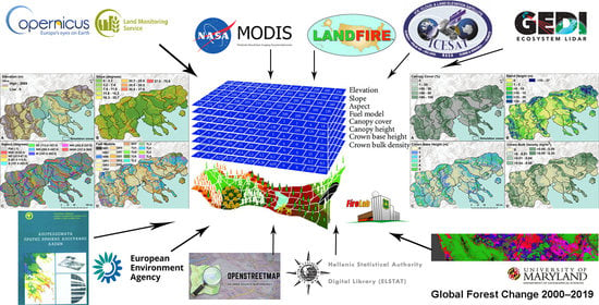
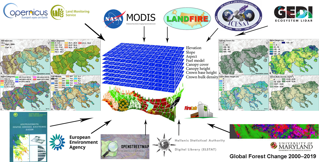
2.1. Data Overview

MTT requires the support of a Geographic Information System (GIS) to generate, manage, and provide spatial data themes containing fuels, vegetation and topography. Five raster data themes are required to run surface fire behavior modelling (elevation, slope, aspect, fuel model and canopy cover). Three additional optional layers describe canopy conditions at the stand level (crown bulk density, canopy base height and stand height). All themes must be co-registered as ascii rasters, with identical resolution, extent, projection, and datum, combined into a single Landscape (LCP) file as required by MTT. Finally, weather and fuel moisture data, and an ignition probability raster are also required. Some of the abovementioned data can be easily retrieved from open-access databases (e.g., topography and weather), while others such as canopy structure and surface fuels require advanced remote sensing (LiDAR), spatial analysis and statistical techniques, in addition to ground-truth data from forest inventories, to be accurately created [43,44,45,46,47,48]. In the US, LANDFIRE provides the required landscape scale geospatial products to support MTT simulations, thus simplifying MTT application. For Europe, a similar system, the Copernicus Land Monitoring Service (hereafter referred as Copernicus), provides a wealth of spatial data and information, although it does not include the entire required dataset for MTT runs.

2.2. Study Area

During a fire simulation, if the spatial domain of the abovementioned themes is limited inside the study area boundaries, then an “edge effect” will appear that will not permit incoming and outgoing fires from and to the study area to be modelled uninterrupted, i.e., all fires will stop at the edges of the domain, creating a “false” barrier to fire spread. To avoid this effect, we created a 10-km buffer around the study area (the Greek region of Macedonia with an area of 34,000 km2) that included parts of Albania, North Macedonia, Bulgaria, and the Greek regions of Thrace, Ipiros and Thessaly (Figure 1A). This buffer zone was integrated with Macedonia.
Then, the buffered study area was divided into seven fire regime macro-areas according to the climatic stratification of the environment by Metzger [49], and adapted to watershed and local municipality boundaries (Figure 2). The most extensive climatic stratification of the environment class is the “Warm temperate and mesic” covering 1.5 million ha, mostly across the coastal zone and large river valleys, followed by the “Cool temperate and xeric” with 860,000 ha on the large plains of western Macedonia, the “Cool temperate and dry” with 625,000 ha being dominant on all mountain ranges, and the ”Warm temperate and xeric” with 570,000 ha on the large plains of central and eastern Macedonia. The remaining three classes are dominant on higher altitudes, covering altogether 660,000 ha. The average macro-area size is 610,000 ha, with the largest covering 900,000 ha and the smallest 460,000 ha.
These macro-areas were further internally subdivided into 30 simulation zones to better capture the fire-weather variability and account for differences in local winds by using more weather stations, each with a smaller area of influence and with similar geo-physical characteristics (see Figure 1A—dashed red lines). For this, we ensured that each zone was assigned at least one representative remote automatic weather station (RAWS) with at least 10 years of recorded data (triangles in Figure 1A). Data were retrieved from RAWS operated by the National Observatory of Athens, the Hellenic National Meteorological Service, the Forest Research Institute, as well as private companies (ScientAct).

2.3. Vegetation

The CORINE Land Cover (CLC) [50] inventory (2018 version) was the base layer for vegetation mapping (Figure 1A). One drawback of CLC is that it lacks vegetation species types, e.g., all conifer species are lumped into a single class. We intersected the main forest related classes, i.e., Broad-leaved forest, Coniferous forest, Transitional woodland-shrub and Mixed forest, with a detailed vegetation species layer produced by the First National Forest Inventory of Greece (NFIG) that captured the species distribution and cover for reference year 1992. Although outdated, it was the best available indicator of which vegetation species were dominant inside the broad forest category boundaries of CLC. The CLC polygon boundaries were preserved, and a new class was created with the Identity tool in ArcGIS 10.2.2 that contained information for both layers, e.g., conifer forest-Pinus halepensis. In addition, we retrieved up-to-date (i.e., post ca. 2012) vegetation maps for important managed forests of Macedonia created with remote sensing techniques and forest inventories by private contractors, requested by local Forest Service branches that manage each forest. When high accuracy layers were available, they were used to erase the combined CLC and NFIG base layer and then append their vegetation classification, after homogenization of their class names. The most common species found in the study area were Quercus spp. (15.1% of the total area), Fagus spp. (6.95%), Pinus nigra (2.5%), Pinus halepensis (2%), Castanea sativa (0.6%), Pinus sylvestris (0.6%), Pinus leucodermis (0.3%), Juniper spp. (0.1%) and Abies spp. (0.1%) (Appendix A Figure A1).

2.4. Land Tenure and Ownership

The land tenure and ownership layer describes how the landscape is partitioned into different forest management regimes, a necessary layer to derive cross-boundary fire transmission estimates (Figure 1B). The CLC layer contains information about basic land uses, which was used as our base mapping layer. The first new classes added to the base mapping layer were community cores and WUI (see Section 2.6). Next, we added ownership information using six major landowner classes, i.e., state, municipal, community, church, private and cooperative for all forested areas with an official forest management plan. Where ownership information was absent, we preserved the original CLC classification. Finally, we retrieved the nationally designated areas from the European Environment Agency [51] with information about protected areas. There are several different types of protected areas and we kept only those where legislation prohibits any form of vegetation management (e.g., national forest or park cores, natural protected areas, aesthetic forests, etc.). Protected area boundaries were used to flag polygons in the base mapping layer where management is restricted.

2.5. Topography

Themes describing topography include elevation, slope and aspect (Figure 3A–C). Elevation is necessary for adiabatic adjustment of temperature and humidity (Figure 3A). The slope theme is necessary for computing direct effects on fire spread and, along with aspect, for determining the angle of incident solar radiation to adjust fuel moisture and for transforming spread rates and directions from the surface to horizontal coordinates [16]. We retrieved the EU-DEM v1.1 from the Copernicus portal [52]. Using GIS, we calculated slope in degrees and aspect in degrees from north.

2.6. Community Areas and Wildland-Urban Interface

Community areas were initially delineated based on CLC urban areas, referred to as continuous and discontinuous urban fabric. To incorporate official census designated boundaries and data defined by the Hellenic Statistical Authority (HSA) including population, number and type of structures, construction material etc., we used the HSA polygons and modified them with the boundaries of the CLC layer. This resulted in a community layer that covered the entire built-up area of the continuous and discontinuous urban fabric. The HSA polygons do not include the expansion of urban areas during the past decade, nor other unofficial urban areas such as residences for tourists. By combining the HSA polygons with the 2018 CLC urban areas, we ensured that all artificial surfaces with a substantial urban footprint were included. These polygons defined the community cores.
To delineate the wildland-urban interface (WUI), which is a zone of transition between wildland and human development, we retrieved the European Settlement Map (ESM) from Copernicus (circa 2017) that maps human settlements in Europe based on SPOT5 and SPOT6 satellite imagery and represents the percentage of built-up area coverage per spatial unit. All pixels that were flagged as build-up areas (i.e., buildings, green urban atlas, green NDVIx and Open Space) were converted into polygons subtracting community cores (see Appendix A Figure A2). The remaining polygons were characterized as the WUI after deleting all spatially isolated and small polygons (<1 ha) at a distance > 2 km from the nearest community core.

2.7. Surface Fuel Models

A surface fuel model is a stylized set of fuel bed characteristics and, depending on local conditions, one or several fuel models may be appropriate (Figure 3D). We adapted and converted the detailed classes of both dominant cover types and species from the vegetation layer (Figure 1—species not shown for mapping purposes) into fuel model codes based on the Scott and Burgan [53] classification system. In total, we used 18 fuel model codes (Table 1).
Initially, we resampled the ESM Built-up area 10-m cells (release 2019) into 100-m raster cells and assigned the non-burnable fuel model NB1. Next, the Copernicus ploughing indicator (circa 2018), which maps the number of years since the last indication of ploughing (1–6), was resampled into a 100-m raster and was assigned with the non-burnable fuel model NB3 to describe non-burnable agricultural lands.
Grasslands burn differently across the elevation gradient, with higher altitudes being moister and with different plant properties, i.e., density, height, mixture with shrubs, dead fuel moisture of extinction and curing period. We combined the Copernicus grasslands (Figure 4), i.e., binary status layer mapping grassland and all non-grassland with 10 m cell size (circa 2018), with the DEM to assign a different grass or grass-shrub fuel model based on elevation classes from past research by the authors and other relevant publications [54,55]. For altitudes up to 800 m, where summers are long and dry, we assigned two grass-shrub fuel models: 0–300 m, GS1 (low load, dry climate grass-shrub); 300–800 m, and GS2 (moderate load, dry climate grass-shrub). For altitudes above 800 m, with short summers and occasional rainfall, we assigned four grass fuel models: 800–1200 m, GR7 (high load, dry climate grass); 1200–1600 m, GR4 (moderate load, dry climate grass); 1600–1800 m, GR5 (low load, humid climate grass); and >1800 m, GR3 (low load, very coarse, humid climate grass).
Lastly, using the University of Maryland Forest Loss per Year data [56] we retrieved the locations of pixels that faced forest loss during 2019 and assigned the fuel model GS1 (Figure 4). Since the CLC is for the reference year 2018, it was crucial to account for forest losses occurring after 2018.

2.8. Forest Canopy Characteristics

Tree cover was retrieved from the Copernicus portal, showing the level of tree cover ranging from 0 (all non-tree covered areas) to 100% for the reference year 2018 in 10 m spatial resolution (Figure 5A). For stand height (Figure 5B), we retrieved the Global Ecosystem Dynamics Investigation (GEDI) Level 3 (L3) gridded mean canopy height (1 km spatial resolution) [57], which was resampled at 100 m. GEDI produces high resolution laser ranging observations of the 3D structure of the Earth using a LiDAR sampling instrument mounted on the International Space Station since late 2018. Data gaps for certain parts of the study area were covered with LiDAR canopy height estimations from the Geoscience Laser Altimeter System instrument aboard ICESat (ca. 2005) [58].
We used data from field inventories and local/expert knowledge to assign species specific constant values for crown base height (in meters) (Figure 5C). For crown bulk density we used lookup tables (Table 2 in Keane et al. [59]) that described the available canopy fuel for a fire to consume in kilograms per cubic meter for common North American tree species and for three canopy cover classes (Low: 21–50%; Medium: 51–80%; High 81–100%). We matched North American species to similar tree species in our study area based on similarity of characteristics, families, and traits (one value for each species), and then we modified canopy fuel values for each of the three canopy cover classes (Figure 5D).

2.9. Probability of Ignition

MTT fire simulation programs can use an ignition probability grid ranging from 0 to 1 to place ignitions across the simulation landscape. First, the recorded ignitions from 1985 to 2000 were retrieved from previously published work [60]. We also retrieved and merged the active fire data from MODIS and VIIRS satellites, covering the period 2000–2019. Since VIIRS has a temporal coverage from 2012, we removed duplicate records and points from the same fire event (one fire event has multiple points in the original dataset) (Figure 6A).
To account for potential ignition locations that have not yet occurred, we used the OpenStreetMap road network layer, and we created a 20-m buffer on each side of major roads, since proximity to roads correlates with fire occurrence [61]. In addition, since the spatial configuration of development patterns influence wildfire ignition [62], we created a 500-m outer buffer around community cores. Within the road network buffer, we randomly allocated 5000 points with a minimum allowed distance of 200-m between points (Figure 6B), while within the community buffer we allocated 6000 points with 300-m minimum distance (Figure 6C). The full dataset contained more than 18,000 points and we created a Point Density raster with ArcGIS, setting a 5-km search radius (i.e., smoothing) to ensure that all burnable pixels will have a value > 0 that allows an ignition to randomly occur there during wildfire simulations, even with a very small probability, except for those pixels assigned with a non-burnable fuel model. Finally, we rescaled the resulting layer to a 0–1 range (Figure 6D).

2.10. Weather Data

For each RAWS, we estimated the frequency of the dominant wind directions and used it as the base for each simulation scenario, with frequency translated into scenario selection probability. The average wind gust speed for each RAWS was used as the base wind speed for all simulations (to be modified during the calibration phase—see next section) since large human-caused wildfires (>50 ha) are typically influenced by higher wind speeds thus increasing rapidly in size [12]. Finally, using the average and highest recorded temperature and relative humidity, we defined the temperature range to be used in the Fine Dead Fuel Moisture Calculation Tool of BehavePlus to estimate the dead fuel moisture content. All weather estimates covered only the months of July and August, which are the most critical months based on the historical ignition data of the past 20 years in terms of both ignition frequency and large wildfire occurrence. For the zones with two or more RAWS, we merged their records to create a single fire simulation scenario file. In total we created 30 scenario files, one for each simulation zone, each with typically eight sets of simulation parameters that include wind speed and direction, duration, fuel moistures, probability of selection and spot probability (see Appendix A Table A1).
We set a constant value for spot probability across all simulation zones and for all scenarios. Spotting probability estimates how many crown fire initiation nodes will launch embers that can start a new fire. Based on communication with Fire Service chiefs within the study area, we learned that spotting is very common for wind-driven fires that ignite during July and August, and very often result in new fires. To account for this high spotting frequency, we set a high spotting probability value (0.25—i.e., one out of the four nodes with crown fire behavior) for simulation zones that are close to coast areas or covered with low elevation conifers and dense shrublands, and lower values for the more elevated zones, mostly covered with broadleaf vegetation. Spotting probability >0.25 was avoided since launching embers from every crown fire node (value = 1) can be computationally intensive, resulting in a long running simulation which often does not change results (as explained in the FlamMap 6 manual).

2.11. Wildfire Simulations and Model Validation

MTT is a state-of-the-art fire-growth modelling algorithm that can model fire behavior on complex landscapes by searching for the minimum time for fire to travel among nodes in a two-dimensional network, interpolated to reveal fire perimeter boundaries and behavior characteristics (e.g., spread rate, fireline intensity). MTT allows simulation of thousands of potential ignitions but without considering vegetation succession or fire suppression. In this study, Monte Carlo simulations were conducted with FConstMTT [19] using an LCP at a spatial resolution of 90 m after resampling all inputs with the nearest neighbor technique. Simulations generated fire perimeters and raster estimates of annual burn probabilities (BP) and conditional flame length (CFL). The annual BP is the ratio of the number of times a pixel burned to the total number of fires simulated, while CFL measures the expected flame length given a pixel burn.
Fire ignitions were initially distributed within the modelling domain according to the ignition probability grid. Then each fire was independently modelled considering a set of simulation parameters, based on the set’s probability of selection, from the scenario file of the simulation zone in which the ignition occurred. In total, 10,000 fires were simulated for each simulation zone, i.e., 300,000 for the entire study area. Initially, we set a base simulation duration of 300 min (five hours of active burning under invariable wind speed and direction).
We performed several iterations of fire modelling for each zone by modifying wind speed (from 25 to 40 km/h) and fire duration (ranging from 60 to 210 min), a necessary step to achieve the best possible calibration. Model calibration was achieved by matching historical and simulated large fire size (>50 ha) distributions at the scale of macro-areas (and not zones), since in most cases the sample of historical fires from each zone was very small (<10 large fires during the past 20 years) (Appendix A Figure A3). For fire simulation modelling, weather conditions were held constant, and fire suppression efforts were not considered due to relatively limited containment capabilities during extreme fire events.

2.12. Community Exposure and Firesheds

First, simulated fire perimeters were used to estimate community exposure by intersecting them with community polygons with the associated total structure density (houses per km2) as recorded by the official HSA census data. Community exposure estimates were calculated as the product of the proportion of area of each community polygon burned by all fires simulated and the structure density for that polygon. This process is a part of an ArcGIS toolbox called XFire [63], used by the authors in previous studies to calculate the community layer intersection with each fire perimeter individually using low level ArcObjects, and estimate the spatial scale and complexity of wildfire exposure in relation to the geography of land tenures [64].
Community exposure values were annualized by estimating the number of years it takes in the region under current annual burned area rates to match the total simulated area burned. In detail, during 2000–2019 the region experienced on average 24.5 incidents per year burning >50 ha each, resulting in 5100 ha area burned annually. The 300,000 simulated fires resulted in 28.5 million ha of burned area (the same pixel can be burned multiple times since each simulation is independent from the others and no change occurs in fuels and stand conditions after it finishes). We estimated that it takes approximately 5600 years (i.e., simulated fire seasons, not actual years) with the current annual burning rate to match the simulated total burned area, thus, annualized values occurred by dividing the structure exposure metrics by 5600.
Finally, the number of structures exposed annually was assigned to each simulated fire ignition, estimating its influence on each community (one ignition to many communities) using GIS analysis. We applied the Inverse Distance Weighted interpolation with a fixed search radius distance of 1 km and 100 m cell size on these ignitions to generate community firesheds.

2.13. Spatial Scale and Complexity of Wildfire Exposure

The estimated spatial scale and complexity of wildfire exposure in relation to the geography of land tenures was estimated with four metrics [64]. Two of these metrics (Source Fire Complexity and Incoming Fire) illustrate the complexity of wildfire exposure in relation to the geography of land tenures. The Source Fire Complexity estimated the number of unique land tenures (including communities) that contributed fire to a given pixel. The Incoming Fire metric measured the percentage of incoming area burned to each pixel, that is, from an ignition outside the land tenure parcel (i.e., a different land tenure) versus self-burning fire from ignitions inside the land tenure parcel, averaged across all fires. The other two metrics (Fire Size Arrival and Fire Size Potential) illustrate the scale of simulated fire size. The Fire Size Arrival metric measured the average fire size (ha) that burned each pixel. Finally, the Fire Size Potential metric estimated the average fire size (ha) generated by ignitions in each pixel. These four metrics can answer questions such as “where do simulated large fires start?”, “which parts of the landscape are affected by the largest simulated fires?”, “where are cross-boundary wildfires predicted?” and “how many different land tenures contribute to the exposure of a given location?”.

3. Results

Burn probability (BP; number of times a pixel burned per 10,000 simulated ignitions) estimates revealed that 25% of the study area did not burn by any simulated fire, while 17% burned from only one fire (Figure 7A). A large portion of the landscape (42%) burned at a moderate frequency and encountered between 2 and 10 simulated fire events. Locations with very high (>30 times) and high (between 11 and 30 times) burning frequency represented 2% and 14% of the landscape, respectively. These results revealed that 42% of the landscape will either not burn at all or was only burned once, and the question that follows is whether these pixels have not received enough ignitions or the fuel, weather and topographic conditions that prevail at these locations/pixels do not allow fires to spread or become large events. The analysis of fuel model composition for these pixels can be found in Table 2. We also estimated how many of the 300,000 simulated fires occurred in pixels that burned none or once. We found that 11,226 simulated ignitions occurred in pixels that were not burned (3.7% of all simulated ignitions) and 61,050 on pixels that burned once (20.4% of all simulated ignitions). We found that the conditions occurring in certain locations did not allow the ignitions to initiate or become large enough to burn nearby pixels, rather than issues with ignition density.
Estimated conditional flame length was very high (>3 m) on 14% of the study area (Figure 7B and Table 3) which may increase the complexity of fire suppression efforts, probably requiring indirect tactics to confront the fire on those portions of the landscape due to high fire intensities and growth. Most of the area (77%) has the potential to experience low flame lengths (0–2 m), meaning that hand crews and machinery can confront the fire. Finally, 9% of the study area has the potential to experience fires with moderate flame lengths (2–3 m), requiring aerial means in collaboration with ground forces for fire suppression.
Results for BP and conditional flame length are in alignment with what we expected based on fuel models assignment to the different vegetation types, most of which did not produce extreme fire behavior (see Table 1). In the Appendix A Figure A1, the vegetation types that create the most intense wildfires (conifers, sclerophyllous vegetation, and chaparral) cover only 18% of the total study area. On other vegetation types that dominate the landscape, simulated fires were either small and low intensity or large and low-to-moderate intensity (e.g., on pastures, oak or deciduous shrubs).
Simulations revealed a region with predicted high values for both BP and CFL in the mountainous parts of Kozani. Chalkidiki also produced high BP values with moderate-high fire intensity, an expected outcome based on recent fire activity in the region. Finally, parts of Serres, Kavala and Drama produced high BP with moderate-low estimated fire intensity.
The four wildfire exposure metrics (Figure 8) revealed high values for the same parts of the study area for wildfire exposure and complexity. Approximately 60% of the study area (Figure 8A and Table 3) received fire from one or two land tenures, 25% from three or four land tenures and the remaining area (15%) with five or more land tenures, indicating high fire complexity associated with different actors, vegetation types and management practices. The parts of the study area that received the largest fires are covered mostly with sclerophyllous vegetation and grasslands (pastures), while the smallest fires burned in landscapes covered with broadleaf forests, oaks, and agricultural lands (Figure 8B). We found that 20% of the landscape received fires ignited on a different land tenure greater than 75% of the time. In other words, only 25% of all fires simulated to burn that pixel originated from the same land tenure (Figure 8C). So, 60% of the landscape receives less than 50% of its fire from other land tenures, i.e., most fires that burn those pixels come from the same land tenure. Finally, Fire Size Potential shows where we expect the largest fires to ignite, with the highest values found mostly in shrublands and coniferous forests (Figure 8D).
The extent of the fireshed for the approximately 2200 communities of the study area was 8350 km2, i.e., ~27% of the total study area. In Figure 9, we show with warmer colors the locations where potential ignitions can have a large impact in terms of estimated structure exposure on neighboring communities, while colder colors denote either lower structure exposure or low structure density of the exposed communities. Over one percent of the landscape was estimated to be the source of very high exposure to communities, 2.6% high exposure, 4.3% moderate exposure and approximately 9.5% for low and very low exposure classes (Table 3). Higher community exposure was estimated for the prefectures of Kavala, Thessaloniki and Pieria, along with the island of Thasos and the westerns parts of Chalkidiki (Figure 9). The western prefectures of Macedonia experienced lower estimated structure exposure (e.g., Grevena, Kastoria, Florina), probably due to lower population density, smaller extent of WUI and denser community cores.
By combining the levels of exposure and their distances to community boundaries we found that the average distance to communities decreased as exposure increased, i.e., for very high exposure 1.1 km, for high 1.8 km, for moderate 2.3 km, for low 2.9 km and for very low 3.6 km (Table 3). This indicates that in general, high structure exposure fires start close to communities (<3 km) before reaching community boundaries. Results also revealed that wildfires that exposed the highest number of structures occurred near the communities of Chalkidiki (Kassandra), Kozani, Kavala, Serres and the WUI of Thessaloniki; and predicted that 137 structures were exposed each simulated fire season (Figure 10A). Based on data derived from the largest 200 fires (of 300,000 total) in terms of final perimeters (Figure 10B), the smallest fire burned 1832 ha, the largest 3472 ha, and mean fire size was 2150 ha.
Communities with dense cores and relatively small WUI, frequently located on mid-elevation plains and agricultural areas (300–800 m a.s.l.), represent the most common community fire exposure archetype. Simulation results revealed that these communities are at low fire risk and when fires reach their boundaries, they are usually of low to moderate fire intensity. The second most frequent community archetype is found in coastal areas (<300 m a.s.l.) with expanded WUI due to tourism and vacation housing, usually at the interface of forested landscapes comprised of low-elevation conifers and shrubs, that are the most exposed communities and prone to sustaining fire spread burning at higher intensity based on simulation results. Finally, a third archetype includes mountainous (>800 m a.s.l.) rural communities, mostly located in the western part of the study area. These communities are intermixed with high-elevation cold-tolerant forested landscapes, which experience very infrequent stand-replacing fires or low intensity surface fires. An important structural property of all communities in the region of Macedonia is that houses are mostly made of reinforced concrete or are older buildings (100–200 years) constructed with stone walls and ceramic roofs, characteristics that make these structures more fire resilient compared to wooden structures typically found in the US.
One of the key outputs from the post-processing of simulated fire perimeters is the ability to estimate structure exposure and rank a set of communities to identify which are the most exposed and in which parts of their boundary we expect fires to burn. In Figure 11A we show a graph of the top-10 most exposed communities in Macedonia, and their location (Figure 11B). The graph also shows the sources of exposure for each community. In the Appendix A Figure A4 the same information is provided but for the top-50 most exposed communities. Major sources of exposure include other communities and their WUI, sclerophyllous vegetation, agricultural lands with significant areas of natural vegetation and other private agricultural lands. Those communities, largely exposed from ignitions on coniferous forests, transitional woodland-shrub and sclerophyllous vegetation (e.g., Panorama Thessaloniki, Nikisiani, Kokkinoxoma, Peyka) are expected to experience more intense wildfires, either due to very flammable canopy fuels or from dense surface fuels.

4. Discussion

4.1. Application and Expansion to Other Regions

Our framework provides a relatively straightforward process that public and private entities concerned with wildland fire management can apply to advance the assessment of wildfire risk and hazard in fire prone regions of Europe. The framework uses publicly available datasets that cover extensive areas with published accuracy assessments (e.g., Copernicus). Thus, researchers in other areas where wildfire simulation modelling is data limited can adopt the methods for their locale, thereby reducing the cost of data acquisition and simplifying complex post-processing. For the application of the proposed framework, familiarity with open-access tools and models such as ArcFuels [65], FConstMTT [19,36] and XFire [64] is required to perform Monte Carlo fire simulations and post-process the results. The use of Monte Carlo wildfire simulations coupled with underlying fire size probability distributions allows the assessment of extreme and rare fire weather conditions and ignition locations, exposing future plausible wildfire disasters.
The application of the framework requires careful calibration within multiple model components to achieve robust results. First, fuel model assignment from Corine or other similar products that group vegetation species into broad vegetation types (e.g., pine, spruce, cedar and fir species as “coniferous forests”) requires that these general types be classified as different species. Our approach used a polygon layer depicting the dominant area of each species and merged it with the boundaries of the Corine layer. This can be accomplished with the “identity” command in ArcGIS, maintaining the outer boundary of a Corine polygon of broad vegetation type (e.g., conifers) while assigning species information within its boundaries. When fuel models are assigned, an important consideration is that fuel conditions are not constant even within the same species area, and variations exist from different management and disturbance histories of each stand. For example, we consistently noticed that fuel conditions in olive groves varied depending on the amount of income they provide to their owners and to the level of land abandonment, ranging from non-burnable tilled soil to continuous grass-shrub fuel or a chaparral understory [1]. As a result, olive groves cannot be described with a single fuel model. A field assessment with visual estimates of the dominant fuel condition can help to better assign fuel models, taking geo-located photographs at frequent intervals along the roadside on a predefined route that intersects and crosses most of the study area.
Most of the required spatial layers describing fuels are of acceptable accuracy for large scale risk and exposure assessments (see the relevant references we provided in each of these datasets in the Materials and Methods), with the exception of canopy base height and crown bulk density. In our case, an independent accuracy assessment would be beneficial for these two layers, but we lacked accurate ground truth data to accomplish this task and it was beyond the scope of this paper. In places where LiDAR data are available there are several different methods that can be applied to create these two layers, but for most cases indirect methods and expert knowledge are required to estimate them. Both metrics are highly variable in real conditions and the assignment of a single value for each species can substantially under- or overestimate them. For canopy base height, in cases where field inventory plots of geo-located photographs are available, they can be used to correct the estimates, but since these datasets are both of limited extent and hard to retrieve, the only alternative is to contact experts in the field of forestry and use their knowledge to create a lookup table for each species, then assign a constant value to it. Forest management plans can also provide useful information if they are available. Crown bulk density is a complicated metric to estimate, since it is a representation of all canopy fuel that can be consumed during a fire (smaller diameter twigs and foliage), and non-destructive field measurements that can be used to calculate it at the stand-level are time-demanding and costly. To our knowledge, we used the best available approach by matching the values of North American species found in Table 2 of Keane et al. [59] with species from the same family within each study area, while accounting for their canopy cover. In this way, value variability is maintained since for each species we do not use a single value but rather, three for each canopy cover class (low, medium and high). The same lookup table provides another distinction for each species based on their growth (small or medium/large) and whether they belong to an open or closed woodland. Knowledge gained from previous research efforts can also be used to assess canopy base height and crown bulk density. In particular, stereo photographs, hemispherical photographs, and stand data for five Interior West conifer stands were used to associate them with biomass estimates and canopy fuel characteristics in order to help fuel managers estimate canopy fuel characteristics in similar forest conditions [66]. Finally, it is important to correct for disturbances to canopy characteristics and structure with the latest available data [56].
Historical fire location, size and typical duration are among the most important inputs that inform simulated ignition locations and fire size distributions. We acknowledge that many countries/regions do not have accurate records of these data and have only recently started to geo-locate each fire ignition. Using MODIS satellite datasets, fire hot-spots can be used to reconstruct historical ignitions with high accuracy, but often multiple records exist for the same fire, especially when it becomes a large-scale event. These datasets also do not provide important information about each event, such as final fire size. As a result, it is time-consuming to verify each hot-spot and assign validated information recorded from fire suppression agencies. At a minimum, cleaning MODIS-derived datasets for multiple records for the same fire event and keeping only the earlier record is necessary. To ensure that fire ignitions are simulated in areas that do not have recorded ignitions, we randomly allocated ignitions across roads and on the periphery of populated places such that one-third of the total ignitions belonged to satellite-derived hot-spots, one-third across roads, and the rest close to populated places. Historical fire sizes are well documented in Europe since 2008 by EFFIS [67]. Although most fire management services in Europe do not use geo-spatial information to map burnt areas, they do have estimates of total burnt area and the name of the place where the fire started and burned. If this information is retrieved, then it is possible to create historical fire size distributions for each simulation macro-area, and then validate Monte Carlo fire simulation results. Fire duration is also an important input to control wildfire simulations and can be inferred by excluding periods during a day when active fire spread is limited or the wind is blowing at low speeds (e.g., late evening to late morning).
Capturing representative weather in simulations requires a decadal time-series record, with hourly intervals. When several stations are available, separate analysis can be conducted for each station and the results merged to identify wind direction frequency. In case a designated sensor to measure 10-hr fuel moisture is not available for a weather station, it can be estimated by providing basic topographic features of the study area, relative humidity and air temperature in the Fine Dead Fuel Moisture Tool of BehavePlus [68]. Another consideration is the length of the fire season, which in our case was the months of July and August. If large wildfires are frequent in a study area during e.g., May or September, these months should also be included in the weather data analysis.
Community areas can be accurately delineated from a combination of Corine and satellite-derived data, but during fuel model assignment non-burnable parts should be identified from the ESM Built-up area dataset and flagged as appropriate. Wildland–urban interface boundaries should be as inclusive as possible containing all areas around communities with structures intermingled with vegetation. Recent studies [27,37] showed that building locations can be obtained for sources such as Open Street Maps [69] or Microsoft Bing Map Building Footprints [70] (not available yet for Europe), providing a more accurate estimate of the number of structures within each community (compared to the census estimated structure count we used in this study) and the location of residential housing, commercial buildings, farms, large stores, industrial buildings, and religious structures.

4.2. Improving Community Protection Using Fire Simulation

The wildfire simulation methods we used account for probabilistic ignition locations and subsequent fire spread under assumed weather and generate multiple outputs useful for understanding the likelihood of extreme events and their impact [40]. This information can be used for improving the planning, mitigation, and adaptation in fire prone landscapes [71]. In the absence of an analytical framework like that described in this paper, it would be difficult to estimate exposure at the community scale and understand how different land ownerships affect fire spread and intensity in and around populated areas. Burn probability and intensity estimates from fire simulations can be used in a wide range of mapping and prioritization processes to help allocate funding for wildfire risk reduction. Fire simulation models can reduce the uncertainty associated with fire management planning by identifying large and rare plausible events.
It is important to note that this study estimated exposure to structures but did not predict building loss. On average, in places like the western US about 20% of the buildings exposed to fire are also destroyed, providing a coarse way of estimating loss from exposure. Landscape fire simulation models cannot predict and model building ignition from firebrands or building-to-building ignitions. Potentially, all structures regardless of construction material (concrete, stone, or wood) can be lost, as experienced from past fire events in Greece (2007 and 2018). A number of prior studies have limited their analysis to exposure, which is adequate for prioritizing investments and identifying firesheds around developed areas [26,27,64], especially where most structures are wooden.
As a proof of concept, we provided in Figure 12 one satellite photo for each of the top-10 most exposed communities to illustrate the different typologies of communities and WUI in Macedonia and the vegetation types associated with fire spread inside community boundaries. In Figure 12A, the Thessaloniki interface WUI is clearly delineated, neighboring a dense Pinus halepensis forest to the east. In Figure 12B, the Panorama Thessalloniki intermix WUI shows structures intermingled with dense stands of conifers in the north. In Figure 12C, a typical rural community in western Macedonia (Siatista), although not adjacent to conifer or broadleaf forest, receives large amounts of transmitted fire from open spaces with little vegetation, mostly grasses and sparse shrubs. In Figure 12D, the community of Nikisiani (Kavala) is surrounded by dense interface chaparral to the east and west, with agricultural lands to the north and south. In Figure 12E, the coastal town of Thasos with intense tourism development in former agricultural lands, can potentially receive fires from western and southeastern conifer forests (fuel breaks are visible in both conifer stands).
In Figure 12F, the community of Kokkinoxoma (Kavala) is surrounded by broadleaf forests and chaparral, including both interface and intermix WUI, that could be threatened by potential fire events. In Figure 12G, the community of Peyka (Thessaloniki) has a broad interface WUI zone to the southwest, while to the north and east intermix WUI is predominant. In Figure 12H, the community of Nea Skioni (Chalkidiki) is a coastal town mostly exposed to fires coming from the west (transitional woodland-shrub, mostly chaparral), since it borders olive cultivation to the north. In Figure 12I, the small town of Skala Raxoniou on the island of Thasos can be potentially exposed to chaparral fires from the south and northeast. Finally, the tourism community of Akritas Ey Zin in Chalkidiki (Figure 12J) is surrounded by sparse conifers mixed with chaparral, and agricultural areas with significant natural vegetation, mostly short shrubs. From the three dominant community exposure typologies, the dense core and limited-extent WUI type can be found in Figure 12D,F, the expanded WUI type in Figure 12A,B,E,G–J, and the mountainous rural communities in Figure 12C.
Forest management agencies can use these findings to create a fuel management prioritization typology for the communities in the study area. For example, they can select the expanded WUI type communities that are in the list of the top-50 most exposed communities and then filter to those with conifer forests as the source of exposure, excluding others, e.g., surrounded by dense chaparral. Then, a smaller scale analysis can follow considering the fireshed boundary of each of those communities. Within the fireshed, places with both high burn probability and fire intensity could be good candidate sites to receive fuel treatments. Furthermore, locations inside the fireshed that receive fire from several different land tenures could be identified to promote shared stewardship projects among the different landowners. Finally, communities with high percentages of incoming fire may by exposed by fires ignited long distances from community boundaries; while current mitigation planning is applied at very local scales around community boundaries. The sources of exposure for these communities can be identified and fuel treatments can be applied at the ignition source, highlighting the need to modify the business-as-usual approach.

5. Conclusions

Creating model-ready datasets and applying them to analyze wildfire risk and exposure for any European region is a tractable problem if Copernicus data and other datasets from trusted publishers/creators are used in conjunction with local knowledge and auxiliary datasets that describe the forest conditions and the fire history of each area. Careful calibration of fire simulation models is required to generate outputs that withstand critiques from land managers and the scientific community. Our pilot application in Macedonia, Greece, provided a proof-of-concept that showed both the methods to generate wildfire simulation outputs and their interpretation in terms of community protection planning. The results can be used to prioritize government investments and field management programs according to the levels of exposure identified in the study. Our future work will include the expansion of the data to cover all of Greece in order to generate fire simulation outputs for national level prioritization of fuel and fire management activities, as recently done in Portugal [39]. These data will be used to create a National Fireshed Registry [4], as in the US, to delineate fireshed boundaries and identify hotspots of exposure to prioritize fuel treatments and other risk mitigation activities. The results will provide policymakers consistent assessment of wildfire exposure to developed areas in the country to guide future policy development in response to the growing wildfire problem.

Author Contributions

Conceptualization, Palaiologos Palaiologou; methodology, Palaiologos Palaiologou, Kostas Kalabokidis and Alan A. Ager; validation, Alan A. Ager, Michelle A. Day and Kostas Kalabokidis; formal analysis, Palaiologos Palaiologou; writing—original draft preparation, Palaiologos Palaiologou; writing—review and editing, Michelle A. Day, Alan A. Ager and Kostas Kalabokidis; Resources: Spyros Galatsidas and Lampros Papalampros; Investigation: Spyros Galatsidas and Lampros Papalampros. All authors have read and agreed to the published version of the manuscript.

Funding

This research is co-financed by Greece and the European Union (European Social Fund- ESF) through the Operational Programme “Human Resources Development, Education and Lifelong Learning 2014–2020” in the context of the project “Spatial optimization of alternative fuel treatment scenarios for managing fire risk” (MIS: 5048196).

Data Availability Statement

The data presented in this study are available on request from the corresponding author. The XFire ArcGIS toolbox and the command-line fire simulator FConstMTT can be provided upon request to Alan Ager ([email protected]).

Acknowledgments

We would like to thank the Greek Forest Service branches of Drama, Chalkidiki, and Kastoria for providing important forestry data for completing this work. We also like to thank the Hellenic Statistical Authority for providing community related census data.

Conflicts of Interest

The authors declare no conflict of interest.

Appendix A

Figure A1. Major vegetation types in the study area from the combined CORINE Land Cover and First National Forest Inventory of Greece layers. In parentheses, the percentage coverage of each vegetation type is provided.
Ijgi 11 00198 g0a1
Figure A2. Community core boundaries (black outline), as delineated by combining the datasets from the Hellenic Statistical Authority and the Corine land cover Urban Fabric classes, and the Wildland–Urban Interface boundaries (blue outline) delineated from the 2017 European Settlement Map built-up layer that is not part of the community cores.
Ijgi 11 00198 g0a2
Figure A3. Fire modelling calibration by matching historical and simulated large fire size (>50 ha) distributions at the scale of macro-areas.
Ijgi 11 00198 g0a3
Figure A4. (A) The top-50 exposed communities based on simulated structure exposure from wildfires and (B) their location in the study area.
Ijgi 11 00198 g0a4
Table A1. Set of simulation parameters as required by the FConstMTT (scenario file). LH: Live herbaceous moisture; LW: Live woody moisture.
IndexWindspeed (mph)Direction (Degrees)Duration (min)Probability of SelectionFuel Moisture File
(1 h 10 h 100 h LH LW)
Spot
Probability
1191351800.42frakto.fms0.25
119901800.16frakto.fms0.25
119681800.09frakto.fms0.25
119401800.08frakto.fms0.25
1192351800.1frakto.fms0.25
1191131800.05frakto.fms0.25
1191701800.08frakto.fms0.25
1192931800.02frakto.fms0.25

References

  1. Palaiologou, P.; Kalabokidis, K.; Ager, A.A.; Day, M.A. Development of comprehensive fuel management strategies for reducing wildfire risk in Greece. Forests 2020, 11, 789. [Google Scholar] [CrossRef]
  2. Ager, A.A.; Day, M.A.; Short, K.C.; Evers, C.R. Assessing the impacts of federal forest planning on wildfire risk mitigation in the Pacific Northwest, USA. Landsc. Urban Plan. 2016, 147, 1–17. [Google Scholar] [CrossRef] [Green Version]
  3. Charnley, S.; Kelly, E.C.; Wendel, K.L. All lands approaches to fire management in the Pacific West: A typology. J. For. 2016, 115, 16–25. [Google Scholar] [CrossRef]
  4. Ager, A.A.; Day, M.A.; Ringo, C.; Evers, C.R.; Alcasena, F.J.; Houtman, R.; Scanlon, M.; Ellersick, T. Development and Application of the Fireshed Registry; RMRS-GTR-425; USDA Forest Service, Rocky Mountain Research Station: Fort Collins, CO, USA, 2021; p. 47. [Google Scholar]
  5. Duane, A.; Piqué, M.; Castellnou, M.; Brotons, L. Predictive modelling of fire occurrences from different fire spread patterns in Mediterranean landscapes. Int. J. Wildland Fire 2015, 24, 407. [Google Scholar] [CrossRef]
  6. Costafreda-Aumedes, S.; Comas, C.; Vega-Garcia, C. Spatio-Temporal Configurations of Human-Caused Fires in Spain through Point Patterns. Forests 2016, 7, 185. [Google Scholar] [CrossRef] [Green Version]
  7. Vacchiano, G.; Foderi, C.; Berretti, R.; Marchi, E.; Motta, R. Modeling anthropogenic and natural fire ignitions in an inner-alpine valley. Nat. Hazards Earth Syst. Sci. 2018, 18, 935–948. [Google Scholar] [CrossRef] [Green Version]
  8. Elia, M.; D’Este, M.; Ascoli, D.; Giannico, V.; Spano, G.; Ganga, A.; Colangelo, G.; Lafortezza, R.; Sanesi, G. Estimating the probability of wildfire occurrence in Mediterranean landscapes using Artificial Neural Networks. Environ. Impact Assess. Rev. 2020, 85, 106474. [Google Scholar] [CrossRef]
  9. Marcos, B.; Gonçalves, J.; Alcaraz-Segura, D.; Cunha, M.; Honrado, J.P. Improving the detection of wildfire disturbances in space and time based on indicators extracted from MODIS data: A case study in northern Portugal. Int. J. Appl. Earth Obs. Geoinf. 2019, 78, 77–85. [Google Scholar] [CrossRef]
  10. Sifakis, N.I.; Iossifidis, C.; Kontoes, C.; Keramitsoglou, I. Wildfire Detection and Tracking over Greece Using MSG-SEVIRI Satellite Data. Remote Sens. 2011, 3, 524–538. [Google Scholar] [CrossRef] [Green Version]
  11. Li, P.; Xiao, C.; Feng, Z.; Li, W.; Zhang, X. Occurrence frequencies and regional variations in Visible Infrared Imaging Radiometer Suite (VIIRS) global active fires. Glob. Change Biol. 2020, 26, 2970–2987. [Google Scholar] [CrossRef]
  12. Abatzoglou, J.T.; Balch, J.K.; Bradley, B.A.; Kolden, C.A. Human-related ignitions concurrent with high winds promote large wildfires across the USA. Int. J. Wildland Fire 2018, 27, 377–386. [Google Scholar] [CrossRef]
  13. Scott, J.H.; Short, K.C.; Finney, M.; Gilbertson-Day, J.; Vogler, K.C. FSim: The Large-Fire Simulator Guide to Best Practices Version 0.3.1; Missoula Fire Sciences Lab: Missoula, MT, USA, 2018. [Google Scholar]
  14. Bar Massada, A.; Syphard, A.D.; Hawbaker, T.J.; Stewart, S.I.; Radeloff, V.C. Effects of ignition location models on the burn patterns of simulated wildfires. Environ. Model. Softw. 2011, 26, 583–592. [Google Scholar] [CrossRef]
  15. Finney, M.A. An overview of FlamMap fire modeling capabilities. In Fuels Management-How to Measure Success: Conference Proceedings, Proceedings of the RMRS-P-41, Portland, OR, USA, 28–30 March 2006; Andrews, P.L., Butler, B.W., Eds.; U.S. Department of Agriculture, Forest Service, Rocky Mountain Research Station: Fort Collins, CO, USA; pp. 213–220.
  16. Finney, M.A. FARSITE: Fire Area Simulator-Model Development and Evaluation; RMRS-RP-4; USDA Forest Service, Rocky Mountain Research Station: Ogden, UT, USA, 1998; p. 47. [Google Scholar]
  17. Finney, M. Fire Spread Probability (FSPro); USDA Forest Service, Rocky Mountain Research Station, Fire Sciences Laboratory: Missoula, MT, USA, 2002. [Google Scholar]
  18. Finney, M.A.; McHugh, C.W.; Grenfell, I.C.; Riley, K.L.; Short, K.C. A simulation of probabilistic wildfire risk components for the continental United States. Stoch. Environ. Res. Risk Assess. 2011, 25, 973–1000. [Google Scholar] [CrossRef] [Green Version]
  19. Ager, A.A.; Evers, C.R.; Day, M.A.; Preisler, H.K.; Barros, A.M.; Nielsen-Pincus, M. Network analysis of wildfire transmission and implications for risk governance. PLoS ONE 2017, 12, e0172867. [Google Scholar] [CrossRef]
  20. Ager, A.A.; Finney, M.A.; McMahan, A.J.; Cathcart, J. Measuring the effect of fuel treatments on forest carbon using landscape risk analysis. Nat. Hazards Earth Syst. Sci. 2010, 10, 2515–2526. [Google Scholar] [CrossRef]
  21. Finney, M.A.; Seli, R.C.; McHugh, C.W.; Ager, A.A.; Bahro, B.; Agee, J.K. Simulation of long-term landscape-level fuel treatment effects on large wildfires. Int. J. Wildland Fire 2007, 16, 712–727. [Google Scholar] [CrossRef] [Green Version]
  22. Barros, A.M.G.; Ager, A.A.; Day, M.A.; Palaiologou, P. Improving long-term fuel treatment effectiveness in the National Forest System through quantitative prioritization. For. Ecol. Manag. 2019, 433, 514–527. [Google Scholar] [CrossRef]
  23. Salis, M.; Laconi, M.; Ager, A.A.; Alcasena, F.J.; Arca, B.; Lozano, O.; Fernandes de Oliveira, A.; Spano, D. Evaluating alternative fuel treatment strategies to reduce wildfire losses in a Mediterranean area. For. Ecol. Manag. 2016, 368, 207–221. [Google Scholar] [CrossRef]
  24. Ager, A.A.; Day, M.A.; McHugh, C.W.; Short, K.; Gilbertson-Day, J.; Finney, M.A.; Calkin, D.E. Wildfire exposure and fuel management on western US national forests. J. Environ. Manag. 2014, 145, 54–70. [Google Scholar] [CrossRef]
  25. Evers, C.; Ager, A.A.; Nielsen-Pincus, M.; Palaiologou, P.; Bunzel, K. Archetypes of community wildfire exposure from national forests in the western US. Landsc. Urban Plan. 2019, 182, 55–66. [Google Scholar] [CrossRef] [Green Version]
  26. Ager, A.A.; Day, M.A.; Palaiologou, P.; Houtman, R.; Ringo, C.; Evers, C. Cross-Boundary Wildfire and Community Exposure: A Framework and Application in the Western US; RMRS-GTR-392; USDA Forest Service, Rocky Mountain Research Station: Fort Collins, CO, USA, 2019; p. 36. [Google Scholar]
  27. Ager, A.A.; Day, M.A.; Alcasena, F.J.; Evers, C.R.; Short, K.C.; Grenfell, I. Predicting Paradise: Modeling future wildfire disasters in the western US. Sci. Total Environ. 2021, 784, 147057. [Google Scholar] [CrossRef]
  28. Ager, A.A.; Houtman, R.; Day, M.A.; Ringo, C.; Palaiologou, P. Tradeoffs between US national forest harvest targets and fuel management to reduce wildfire transmission to the wildland urban interface. For. Ecol. Manag. 2019, 434, 99–109. [Google Scholar] [CrossRef]
  29. Ager, A.A.; Day, M.A.; Vogler, K. Production possibility frontiers and socioecological tradeoffs for restoration of fire adapted forests. J. Environ. Manag. 2016, 176, 157–168. [Google Scholar] [CrossRef] [Green Version]
  30. Castellnou, M.; Prat-Guitart, N.; Arilla, E.; Larrañaga, A.; Nebot, E.; Castellarnau, X.; Vendrell, J.; Pallàs, J.; Herrera, J.; Monturiol, M.; et al. Empowering strategic decision-making for wildfire management: Avoiding the fear trap and creating a resilient landscape. Fire Ecol. 2019, 15, 31. [Google Scholar] [CrossRef]
  31. Calkin, D.E.; Ager, A.A.; Gilbertson-Day, J.; Scott, J.H.; Finney, M.A.; Schrader-Patton, C.; Quigley, T.M.; Strittholt, J.R.; Kaiden, J.D. Wildfire Risk and Hazard: Procedures for the First Approximation; GTR-RMRS-235; USDA Forest Service, Rocky Mountain Research Station: Fort Collins, CO, USA, 2010; p. 62. [Google Scholar]
  32. Mitsopoulos, I.; Mallinis, G.; Arianoutsou, M. Wildfire risk assessment in a typical Mediterranean wildland—Urban interface of Greece. Environ. Manag. 2015, 55, 900–915. [Google Scholar] [CrossRef]
  33. Palaiologou, P.; Ager, A.A.; Nielsen-Pincus, M.; Evers, C.; Kalabokidis, K. Using transboundary wildfire exposure assessments to improve fire management programs: A case study in Greece. Int. J. Wildland Fire 2018, 27, 501–513. [Google Scholar] [CrossRef]
  34. Mallinis, G.; Mitsopoulos, I.; Beltran, E.; Goldammer, J. Assessing Wildfire Risk in Cultural Heritage Properties Using High Spatial and Temporal Resolution Satellite Imagery and Spatially Explicit Fire Simulations: The Case of Holy Mount Athos, Greece. Forests 2016, 7, 46. [Google Scholar] [CrossRef] [Green Version]
  35. Xofis, P.; Konstantinidis, P.; Papadopoulos, I.; Tsiourlis, G. Integrating Remote Sensing Methods and Fire Simulation Models to Estimate Fire Hazard in a South-East Mediterranean Protected Area. Fire 2020, 3, 31. [Google Scholar] [CrossRef]
  36. Alcasena, F.J.; Ager, A.A.; Bailey, J.D.; Pineda, N.; Vega-Garcia, C. Towards a comprehensive wildfire management strategy for Mediterranean areas: Framework development and implementation in Catalonia, Spain. J. Environ. Manag. 2019, 231, 303–320. [Google Scholar] [CrossRef]
  37. Salis, M.; Arca, B.; Del Giudice, L.; Palaiologou, P.; Alcasena-Urdiroz, F.; Ager, A.; Fiori, M.; Pellizzaro, G.; Scarpa, C.; Schirru, M.; et al. Application of simulation modeling for wildfire exposure and transmission assessment in Sardinia, Italy. Int. J. Disaster Risk Reduct. 2021, 58, 102189. [Google Scholar] [CrossRef]
  38. Oliveira, T.M.; Barros, A.M.G.; Ager, A.A.; Fernandes, P.M. Assessing the effect of a fuel break network to reduce burnt area and wildfire risk transmission. Int. J. Wildland Fire 2016, 25, 619–632. [Google Scholar] [CrossRef]
  39. Alcasena, F.; Ager, A.; Le Page, Y.; Bessa, P.; Loureiro, C.; Oliveira, T. Assessing wildfire exposure to communities and protected areas in Portugal. Fire 2021, 4, 82. [Google Scholar] [CrossRef]
  40. Parisien, M.-A.; Dawe, D.A.; Miller, C.; Stockdale, C.A.; Armitage, O.B. Applications of simulation-based burn probability modelling: A review. Int. J. Wildland Fire 2020, 28, 913–926. [Google Scholar] [CrossRef] [Green Version]
  41. Kelso, J.K.; Mellor, D.; Murphy, M.E.; Milne, G.J. Techniques for evaluating wildfire simulators via the simulation of historical fires using the AUSTRALIS simulator. Int. J. Wildland Fire 2015, 24, 784–797. [Google Scholar] [CrossRef] [Green Version]
  42. Jahdi, R.; Salis, M.; Darvishsefat, A.A.; Alcasena, F.; Mostafavi, M.A.; Etemad, V.; Lozano, O.M.; Spano, D. Evaluating fire modelling systems in recent wildfires of the Golestan National Park, Iran. Forestry 2016, 89, 136–149. [Google Scholar] [CrossRef] [Green Version]
  43. Myroniuk, V.; Kutia, M.; J Sarkissian, A.; Bilous, A.; Liu, S. Regional-Scale Forest Mapping over Fragmented Landscapes Using Global Forest Products and Landsat Time Series Classification. Remote Sens. 2020, 12, 187. [Google Scholar] [CrossRef] [Green Version]
  44. Palaiologou, P.; Kalabokidis, K.; Kyriakidis, P. Forest mapping by geoinformatics for landscape fire behaviour modelling in coastal forests, Greece. Int. J. Remote Sens. 2013, 34, 4466–4490. [Google Scholar] [CrossRef]
  45. Aragoneses, E.; Chuvieco, E. Generation and Mapping of Fuel Types for Fire Risk Assessment. Fire 2021, 4, 59. [Google Scholar] [CrossRef]
  46. Engelstad, P.S.; Falkowski, M.; Wolter, P.; Poznanovic, A.; Johnson, P. Estimating Canopy Fuel Attributes from Low-Density LiDAR. Fire 2019, 2, 38. [Google Scholar] [CrossRef] [Green Version]
  47. Riaño, D.; Chuvieco, E.; Condés, S.; González-Matesanz, J.; Ustin, S.L. Generation of crown bulk density for Pinus sylvestris L. from lidar. Remote Sens. Environ. 2004, 92, 345–352. [Google Scholar] [CrossRef]
  48. Mielcarek, M.; Stereńczak, K.; Khosravipour, A. Testing and evaluating different LiDAR-derived canopy height model generation methods for tree height estimation. Int. J. Appl. Earth Obs. Geoinf. 2018, 71, 132–143. [Google Scholar] [CrossRef]
  49. Metzger, M.J.; Bunce, R.G.H.; Jongman, R.H.; Mücher, C.A.; Watkins, J.W. A climatic stratification of the environment of Europe. Glob. Ecol. Biogeogr. 2005, 14, 549–563. [Google Scholar] [CrossRef]
  50. EEA. Corine Land Cover (CLC) 2018, Version 2020_20u1. Available online: https://land.copernicus.eu/pan-european/corine-land-cover/clc2018 (accessed on 21 February 2022).
  51. EEA. Nationally Designated Protected Areas (CDDA). Available online: https://www.eea.europa.eu/data-and-maps/data/nationally-designated-areas-national-cdda-15 (accessed on 21 February 2022).
  52. Mouratidis, A.; Ampatzidis, D. European digital elevation model validation against extensive global navigation satellite systems data and comparison with SRTM DEM and ASTER GDEM in Central Macedonia (Greece). ISPRS Int. J. Geo-Inf. 2019, 8, 108. [Google Scholar] [CrossRef] [Green Version]
  53. Scott, J.H.; Burgan, R.E. Standard Fire Behavior Fuel Models: A Comprehensive Set for Use with Rothermel’s Surface Fire Spread Model; RMRS-GTR-153; USDA Forest Service, Rocky Mountain Research Station: Fort Collins, CO, USA, 2005; p. 72. [Google Scholar]
  54. Papanastasis, V.P. Species Structure and Productivity in Grasslands of Northern Greece. In Components of Productivity of Mediterranean-Climate Regions Basic and Applied Aspects, Proceedings of the International Symposium on Photosynthesis, Primary Production and Biomass Utilization in Mediterranean-Type Ecosystems, Kassandra, Greece, 13–15, September 1980; Margaris, N.S., Mooney, H.A., Eds.; Springer Netherlands: Dordrecht, The Netherlands, 1981; pp. 205–217. [Google Scholar]
  55. Roukos, C.; Koutsoukis, C.; Akrida-Demertzi, K.; Karatassiou, M.; Demertzis, G.; Kandrelis, S. The effect of altitudinal zone on soil properties, species composition and forage production in a subalpine grassland in northwest Greece. Appl. Ecol. Environ. Res. 2017, 15, 609–626. [Google Scholar] [CrossRef]
  56. Hansen, M.C.; Potapov, P.V.; Moore, R.; Hancher, M.; Turubanova, S.A.; Tyukavina, A.; Thau, D.; Stehman, S.V.; Goetz, S.J.; Loveland, T.R.; et al. High-Resolution Global Maps of 21st-Century Forest Cover Change. Science 2013, 342, 850–853. [Google Scholar] [CrossRef] [Green Version]
  57. Dubayah, R.O.; Luthcke, S.B.; Sabaka, T.J.; Nicholas, J.B.; Preaux, S.; Hofton, M.A. GEDI L3 Gridded Land Surface Metrics, Version 1; ORNL DAAC: Oak Ridge, TN, USA, 2021. [Google Scholar]
  58. Simard, M.; Pinto, N.; Fisher, J.B.; Baccini, A. Mapping forest canopy height globally with spaceborne lidar. J. Geophys. Res. Biogeosci. 2011, 116, G04021. [Google Scholar] [CrossRef] [Green Version]
  59. Keane, R.E.; Mincemoyer, S.A.; Schmidt, K.M.; Long, D.G.; Garner, J.L. Mapping Vegetation and Fuels for Fire Management on the Gila National Forest Complex, New Mexico; US Department of Agriculture, Forest Service, Rocky Mountain Research Station: Ogden, UT, USA, 2000; p. 126. [Google Scholar]
  60. Koutsias, N.; Balatsos, P.; Kalabokidis, K. Fire occurrence zones: Kernel density estimation of historical wildfire ignitions at the national level, Greece. J. Maps 2014, 10, 630–639. [Google Scholar] [CrossRef] [Green Version]
  61. Zambon, I.; Cerdà, A.; Cudlin, P.; Serra, P.; Pili, S.; Salvati, L. Road Network and the Spatial Distribution of Wildfires in the Valencian Community (1993–2015). Agriculture 2019, 9, 100. [Google Scholar] [CrossRef] [Green Version]
  62. Mobley, W. Effects of changing development patterns and ignition locations within Central Texas. PLoS ONE 2019, 14, e0211454. [Google Scholar] [CrossRef]
  63. Ager, A.A.; Bunzel, K.; Day, M.A.; Evers, C.; Palaiologou, P. XFire: Geospatial Framework for Characterizing Transboundary Wildfire Risk to Communities, Unpublished Report. 2015.
  64. Ager, A.A.; Palaiologou, P.; Evers, C.R.; Day, M.A.; Barros, A.M.G. Assessing transboundary wildfire exposure in the southwestern United States. Risk Anal. 2018, 38, 2105–2127. [Google Scholar] [CrossRef] [Green Version]
  65. Vaillant, N.M.; Ager, A.A.; Anderson, J. ArcFuels10 System Overview; PNW-GTR-875; USDA Forest Service, Pacific Northwest Reseach Station: Portland, OR, USA, 2013. [Google Scholar]
  66. Scott, J.H.; Reinhardt, E.D. Stereo Photo Guide for Estimating Canopy Fuel Characteristics in Conifer Stands; RMRS-GTR-145; USDA Forest Service, Rocky Mountain Research Station: Fort Collins, CO, USA, 2005. [Google Scholar]
  67. EFFIS. European Forest Fire Information System. Available online: https://effis.jrc.ec.europa.eu/ (accessed on 21 February 2022).
  68. Heinsch, F.A.; Andrews, P.L. BehavePlus Fire Modeling System, Version 5.0: Design and Features; Gen. Tech. Rep. RMRS-GTR-249; U.S. Department of Agriculture, Forest Service, Rocky Mountain Research Station: Fort Collins, CO, USA, 2010; p. 111. [Google Scholar]
  69. OSMF. OpenStreetMap. Available online: https://www.openstreetmap.org/ (accessed on 21 February 2022).
  70. Microsoft. Computer Generated Building Footprints for the United States GitHub Repository. Available online: https://github.com/Microsoft/USBuildingFootprints (accessed on 21 February 2022).
  71. Miller, C.; Ager, A.A. A review of recent advances in risk analysis for wildfire management. Int. J. Wildland Fire 2013, 22, 1–14. [Google Scholar] [CrossRef] [Green Version]
Figure 1. (A) Broad vegetation types within the 30 simulation zone boundaries and their associated weather stations for the region of Macedonia, Greece. A 10-km outer buffer was applied (area outside the black outline) to account for fire exchange between the study area and neighboring countries or other Greek regions. (B) Combined land tenures and major ownerships.
Ijgi 11 00198 g001
Figure 2. Climatic macro-areas in the Macedonia study area, including a 10-km buffer to account for incoming and outgoing fires.
Ijgi 11 00198 g002
Figure 3. (A) Elevation derived from the EU-DEM v1.1, retrieved from the Copernicus portal. (B) Slope in degrees. (C) Aspect in degrees. (D) Scott and Burgan fuel type models [53]; NB: Non-Burnable; GR: Grass; GS: Grass-Shrub; SH: Shrub; TU: Timber-Understory; TL: Timber Litter. See Table 1.
Ijgi 11 00198 g003
Figure 4. Forest loss for the period 2000–2019, derived from the Global Forest Change dataset [56] and grasslands derived from the Copernicus portal.
Ijgi 11 00198 g004
Figure 5. (A) Canopy cover, derived from the Copernicus portal. (B) Average stand height in meters. (C) Crown base height in meters. (D) Crown bulk density in kg m−3.
Ijgi 11 00198 g005
Figure 6. (A) Recorded ignitions for the period 1985–2000 merged with active fire data from MODIS and VIIRS satellites for 2000–2019. (B) The 5000 randomly assigned ignitions across roads. (C) The 6000 randomly assigned ignitions around community areas. (D) The ignition probability grid, including the 10-km buffered area, as calculated by all ignitions after applying a point density algorithm.
Ijgi 11 00198 g006
Figure 7. (A) Simulated burn probability, which represents the times each pixel experienced a simulated fire over 10,000 simulations; and (B) conditional flame length that measures the expected fire intensity in meters, given a pixel burned, averaged across all simulated.
Ijgi 11 00198 g007
Figure 8. Spatial scale and complexity of wildfire exposure. (A) Source Fire Complexity; (B) Fire Size Arrival; (C) Incoming Fire; (D) Fire Size Potential. See methods for details.
Ijgi 11 00198 g008
Figure 9. Community fireshed as estimated by intersecting simulated fire perimeters with community polygons (cores and wildland–urban interface) and associated level of structure exposure. Warmer colors denote locations where simulated fires were predicted to cause higher structure exposure.
Ijgi 11 00198 g009
Figure 10. Simulated (A) high exposure fires in terms of structures exposed per year and community boundaries, and (B) largest fires in terms of area burned (ha).
Ijgi 11 00198 g010
Figure 11. (A) The top-10 exposed communities based on simulated structure exposure from wildfires and (B) their location in the study area.
Ijgi 11 00198 g011
Figure 12. The top-10 exposed communities in Macedonia. (A) Thessaloniki; (B) Panorama Thessaloniki; (C) Siatista; (D) Nikisiaki; (E) Thasos; (F) Kokkinoxoma; (G) Peyka; (H) Nea Skioni; (I) Skala Raxoniou, and (J) Akritas Ey Zin.
Ijgi 11 00198 g012
Table 1. Fuel model codes by Scott and Burgan [53], ranked by area and percentage of the study area, including the 10-km buffer zone.
Fuel Model CodeDescriptionArea (ha)%Fuel Model CodeDescriptionArea (ha)%
GR1Short, sparse dry climate grass1,165,65427.3GR7High load, dry climate grass115,6022.7
TL6Moderate load broadleaf litter709,88516.6GR4Moderate load, dry climate grass47,6211.1
SH5High load, dry climate shrub583,18613.7TL2Low load broadleaf litter34,4010.8
GS1Low load, dry climate grass-shrub479,70111.2SH7Very high load, dry climate shrub29,3560.7
GS2Moderate load, dry climate grass-shrub296,2186.9GR5Low load, humid climate grass24,8810.6
TU1Low load dry climate timber-grass-shrub212,6175.0GR3Low load, very coarse, humid climate grass18,4370.4
TL9Very high load broadleaf litter193,9364.5TL3Moderate load conifer litter86150.2
NBNon-burnable185,7844.3TU4Dwarf conifer with understory52160.1
TU5Very high load, dry climate timber-shrub157,9423.7TL8Long-needle litter28480.1
Table 2. Fuel model class percentage for all the pixels that burned once or none.
Fuel Model ClassNot Burned (25% of the Study Area)Burned Once (17% of the Study Area)
Non-burnable13%0%
Grass17%39%
Grass-shrub or Chaparral8%18%
Timber-Understory10%11%
Timber-Litter52%32%
Sum100%100%
Table 3. Results for the main metrics produced from post-processing fire behavior simulation outputs.
Burn Probability (percentage of total area affected)
No fire1 fire2–10 fires11–30 fires>30 Fires
25%17%42%14%2%
Conditional Flame Length (percentage of total area affected)
0–2 m2–3 m>3 m
77%9%14%
Source Complexity Index (percentage of total area affected)
1–2 Land Tenures3–4 Land Tenures>5 Land Tenures
60%25%15%
Structure exposure (percentage of total study area)
Low and Very LowModerateHighVery High
19%4.3%2.6%1.3%
Levels of Exposure and Distances to Community Boundaries
Very LowLowModerateHighVery High
3.6 km2.9 km2.3 km1.8 km1.1 km
Publisher’s Note: MDPI stays neutral with regard to jurisdictional claims in published maps and institutional affiliations.

