Dynamic Response Analysis of Long-Span Bridges under Random Traffic Flow Based on Sieving Method

Abstract

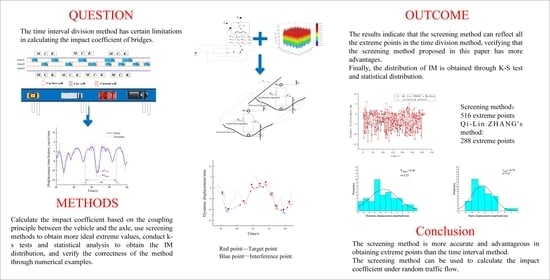
To overcome the limitations of using time interval division to calculate the bridge impact coefficient (IM), a sieving method has been proposed. This method employs multiple sieves on bridge time–history curve samples to ultimately obtain the bridge impact coefficients. Firstly, CA cellular automata are used to establish different levels of traffic flow fleet models. The random traffic flow–bridge coupling dynamic model is established through wheel–bridge displacement coordination and mechanical coupling relationships based on the theory of modal synthesis. Then, the variation of bridge dynamic time–history curves for different classes of random traffic flow, speed and pavement unevenness parameters are analyzed. The sieving method is applied to screen the extreme points of the dynamic time–history curve of the bridge, enabling the distribution law of the bridge IM to be obtained using the Kolmogorov–Smirnov test (K–S test) and statistical analysis. Finally, the calculated value is then compared with the IM specifications of multiple countries. The results show that the proposed method has high identification accuracy and produces a good inspection effect. The value obtained using the sieving method is slightly larger than the value specified in the US code, 0.33, which is considerably larger than the values specified in other national codes. As pavement conditions deteriorate, the IM of the bridge increases rapidly, especially under Class C and Class D pavement unevenness, which exceed the values specified in various national bridge specifications.

1. Introduction

As a crucial component of transportation infrastructure, bridges serve as key nodes in the highway network. Vehicle–bridge coupling vibration affects both the working condition and service life of bridges while also serving as a crucial basis for evaluating the dynamic safety of bridges. Conducting an in-depth study of vehicle–bridge coupled vibration problems is of great significance for the design and safe operation of highway bridges [1,2,3,4,5].

Currently, a reliable, traditional approach to researching vehicle–bridge coupling vibration is to use field tests to obtain bridge dynamic response data for analytical studies. Since the 1950s, a number of field tests have been carried out in countries such as the USA and Australia, providing a reliable basis for the study of vehicle–bridge coupling [6]. However, due to the relatively high cost of field tests and the number of interference factors, it has not been widely used in relevant research [7]. With the rapid development of the computer level, numerical simulation analysis has become the main efficient method for studying vehicle–bridge coupling and has been widely used. Scholars from various countries have used numerical methods to simulate complex multi-degree-of-freedom vehicle–bridge analysis models. Wang et al. [8] established a three-axle vehicle model. Harris et al. [9] and O’ Brien et al. [10] established a five-axle heavy truck model, etc. Some scholars used the distribution function of one or several vehicle models to simulate random traffic [11,12,13], and some scholars assumed random traffic flow as a simpler random process [14,15,16] and used the cellular automaton method [17] or Monte Carlo method (MC) to simulate random traffic flow [18,19,20]. Regarding the simulation of bridge models, it has developed from the one-dimensional beam cell to the two-dimensional plane model [21], then to beam lattice models [22,23,24], three-dimensional solid models [25], etc.

The impact coefficient (IM) is an important indicator for evaluating the dynamic response of a bridge and an important parameter for bridge design and safety assessment. Currently, the traditional IM is determined as the ratio of the dynamic effect to the static effect generated by a vehicle crossing the bridge. However, the actual vehicle load is generated by a random combination of multiple vehicles, and its IM is calculated differently from that of a vehicle. The current mainstream approach for calculating the IM of a bridge under random traffic flow is a method proposed by Qi-Lin Zhang [26], which involves dividing the time periods. The basic principle is to divide the total operating time t of the traffic flow into n small time intervals Δt, analyze the maximum dynamic displacement and maximum static displacement of the bridge within each Δt, and calculate the IM via the ratio of the sample data for the dynamic and static displacement of the bridge [27,28,29]. As shown in Figure 1, the IMs calculated using this method are strongly influenced by the variation of the interval time. However, no reasonable basis for Δt has been provided, leading to significant deviation from the actual situation in the calculated values. Therefore, it is urgent to conduct research on the IM of bridges under random traffic flow.

To address the limitations of the aforementioned research approach, this paper proposes a dynamic analysis model for random traffic–bridge based on the basic principles of the modal synthesis method using cellular automata. Furthermore, a sieving method is proposed for calculating the IM of the bridge based on the extreme value principle, which uses multiple sieving methods for time–history curve samples of the bridge and performs K–S testing and statistical analysis to obtain the IM distribution. This approach offers high accuracy and effective inspection. An IM analysis under random traffic flow is also conducted on a long-span continuous beam bridge as an example. The relevant research results could provide guidance for the calculation and study of such bridges under the influence of random traffic flow.

Using the screening method, which compares the sizes of adjacent points to obtain the extreme points of the bridge structure, allows the shortcomings caused by uneven time division to be avoided, and the obtained extreme points allow for more accurate calculation of the impact coefficient under random traffic flow provided by the screening method. The objective of this work is to calculate the impact coefficient under random traffic flow provided by the screening method.

2. Theory of Random Traffic Flow–Bridge Coupled Vibration

To analyze the coupling effect of random traffic–bridge, a separate dynamical model of random traffic and bridge coupling needs to be developed, and the geometric and mechanical coupling between vehicles and the bridge should be investigated.

2.1. The Vibration Equation of Random Traffic Flow

The vibration equation for random traffic flow is established using the principle of virtual work, as shown in Equation (1).

$$\left\{\begin{array}{l}{\mathit{M}}_v{}_1{\ddot{\mathit{U}}}_{v1}+{\mathit{C}}_v{}_1{\dot{\mathit{U}}}_{v1}+{\mathit{K}}_v{}_1{\mathit{U}}_{v1}={\mathit{F}}_{v1}\hfill \\ {\mathit{M}}_v{}_2{\ddot{\mathit{U}}}_{v2}+{\mathit{C}}_v{}_2{\dot{\mathit{U}}}_{v2}+{\mathit{K}}_v{}_2{\mathit{U}}_{v2}={\mathit{F}}_{v2}\hfill \\ ⋮\hfill \\ {\mathit{M}}_v{}_{(n-1)}{\ddot{\mathit{U}}}_{v(n-1)}+{\mathit{C}}_v{}_{(n-1)}{\dot{\mathit{U}}}_{v(n-1)}+{\mathit{K}}_{v(n-1)}{\mathit{U}}_{v(n-1)}={\mathit{F}}_{v(n-1)}\hfill \\ {\mathit{M}}_v{}_n{\ddot{\mathit{U}}}_{vn}+{\mathit{C}}_v{}_n{\dot{\mathit{U}}}_{vn}+{\mathit{K}}_v{}_n{\mathit{U}}_{vn}={\mathit{F}}_{vn}\hfill \end{array}\right.$$

(1)

Organize Equation (1) into Equation (2):

$${\mathit{M}}_v{\ddot{\mathit{U}}}_v+{\mathit{C}}_v{\dot{\mathit{U}}}_v+{\mathit{K}}_v{\mathit{U}}_v={\mathit{F}}_{bv}$$

(2)

where ${\mathit{M}}_v{}_{\mathrm{i}}$,${\mathit{C}}_v{}_{\mathrm{i}}$,${\mathit{K}}_v{}_{\mathrm{i}}$,${\mathit{F}}_v{}_{\mathrm{i}}$ = the mass matrix, damping matrix, stiffness matrix and external force vector of the ith vehicle, respectively; n is the number of vehicles in the random traffic flow; ${\mathit{M}}_v$, ${\mathit{C}}_v$, ${\mathit{K}}_v$ = the mass matrix, damping matrix and stiffness matrix of the random traffic flow, respectively; ${\mathit{F}}_v$ is the external force vector of the random traffic flow; ${\mathit{U}}_v$ is the displacement matrix of each degree of freedom of the vehicle; ${\dot{\mathit{U}}}_v$ = the velocity matrix of each degree of freedom of the vehicle; ${\ddot{\mathit{U}}}_v$ is the acceleration matrix of each degree of freedom of the vehicle; $F_{bv}$ = the force vector of the bridge on the vehicle.

2.2. The Vibration Equation of Bridge

According to D’Alembert’s principle, establish the vibration equation of bridge:

$$M_b{\ddot{\mathit{U}}}_b+C_b{\dot{\mathit{U}}}_b+K_b{\mathit{U}}_b=F_{vb}$$

(3)

where ${\mathit{M}}_b$, ${\mathit{C}}_b$, ${\mathit{K}}_b$ = the mass matrix, damping matrix and stiffness matrix of the bridge, respectively; ${\mathit{U}}_b$ = the displacement matrix of each degree of freedom of the bridge; ${\dot{\mathit{U}}}_b$ = the velocity matrix of each degree of freedom of the bridge; ${\ddot{\mathit{U}}}_b$ = the acceleration matrix of each degree of freedom of the bridge; $F_{vb}$ = the force vector of vehicle to bridge.

2.3. The Roughness Model of the Road

In this paper, a numerical road roughness model [30] is developed using the harmonic superposition method, wherein the road roughness profile can be represented by the sum of a series of harmonics, as shown in Equation (4).

$$q(x)={\displaystyle \sum _{i=1}^m\sqrt{2G_q(n_{mid-1}\mathrm{\Delta }n)}}\sin (2\pi n_{mid-1}x+{\theta }_i)$$

(4)

where $q(x)$ is the spatial domain dispersion of the wheel corresponding to the road roughness (mm); $G_q$ = the displacement power spectral density (m²/Hz); $n_{mid-1}$ is the central frequency of the ith interval (Hz); $\mathrm{\Delta }n$ = the frequency interval; $n_{mid-1}$ = $\left(i-0.5\right)\mathrm{\Delta }n$; $x$ = the distance travelled by the vehicle (m); θ_i is the random variable from 0 to 2π.

In order to conform to the actual road surface conditions, this paper considers the coherent relationship between the left and right wheels corresponding to road roughness and establishes a spatial road roughness model [31,32,33], as shown in Equation (5).

$${\left({\gamma }^{RL}(n)\right)}^2=\frac{{\left|G_q{}^{RL}(n)\right|}^2}{G_q{}^{RR}(n)G_q{}^{LL}(n)}={\cos }^2({\theta }_i^L-{\theta }_i^R)=co{h}^{2}n$$

(5)

The results of the C-level spatial road roughness surface map are given in Figure 2.

2.4. Vehicle–Bridge Coupling Interaction

2.4.1. Geometric and Mechanical Coupling Relationship between Wheel and Bridge

Assume that, during the driving process, the displacement vector at the centroid of the bridge is ${\mathit{U}}_{bi}$ and the displacement vector at the contact point between the wheel and the bridge deck is ${\mathit{U}}_{vi}$, as shown in Figure 3 and Equations (6) and (7):

$${\mathit{U}}_{bi}=\left[\begin{array}{cccccc}{x}_{\mathrm{b}\mathrm{i}}& y_{\mathrm{b}\mathrm{i}}& z_{\mathrm{b}\mathrm{i}}& {\theta }_{\mathrm{xbi}}& {\theta }_{\mathrm{ybi}}& {\theta }_{\mathrm{zbi}}\end{array}\right]$$

(6)

$${\mathit{U}}_{vi}=\left[\begin{array}{cccccc}{x}_{\mathrm{v}\mathrm{i}}& y_{\mathrm{v}\mathrm{i}}& z_{\mathrm{v}\mathrm{i}}& {\theta }_{\mathrm{xvi}}& {\theta }_{\mathrm{yvi}}& {\theta }_{\mathrm{zvi}}\end{array}\right]$$

(7)

Annotation:

$e$ = the horizontal distance from the centroid of the bridge to the center of the wheelbase (m);

$h$ = the vertical distance from the centroid of the bridge to the center of the wheelbase (m);

B = the lateral distance between the left and right wheels of the vehicle (m);

$m_v$ = body mass (kg);

$\phi$ = roll over moment of inertia (kg·m²);

$K_{\mathrm{Ls}1}$, $K_{\mathrm{Rs}1}$, $K_{\mathrm{Lt}1}$, $K_{\mathrm{Rt}1}$ = suspension stiffness and tire stiffness (kN·m⁻¹);

$C_{\mathrm{Ls}1}$, $C_{\mathrm{Rs}1}$, $C_{\mathrm{Lt}1}$, $C_{\mathrm{Rt}1}$ = damping coefficient and damping coefficient (kN·s·m⁻¹);

$m_{\mathrm{Lx}1}$, $m_{\mathrm{Rx}1}$ = unsprung mass (kg);

$Z_{\mathrm{L}1}$, $Z_{\mathrm{R}1}$ = vertical displacement of suspension system (m);

$x_{\mathrm{b}\mathrm{i}}$, $y_{\mathrm{b}\mathrm{i}}$, $z_{\mathrm{b}\mathrm{i}}$ = the coordinate value at the centroid point of the bridge (m);

${\theta }_{\mathrm{x}\mathrm{b}\mathrm{i}}$, ${\theta }_{\mathrm{y}\mathrm{b}\mathrm{i}}$, ${\theta }_{\mathrm{z}\mathrm{b}\mathrm{i}}$ = the angular displacement at the centroid point of the bridge (°);

$x_{\mathrm{v}\mathrm{i}}$, $y_{\mathrm{v}\mathrm{i}}$, $z_{\mathrm{v}\mathrm{i}}$ = the coordinate value at the point of action of the axle (mm);

${\theta }_{\mathrm{x}\mathrm{v}\mathrm{i}}$, ${\theta }_{\mathrm{y}\mathrm{v}\mathrm{i}}$, ${\theta }_{\mathrm{z}\mathrm{v}\mathrm{i}}$ = the angular displacement at the point of action of the axle (°).

Based on the geometric coupling relationship between wheels and bridge, establish the displacement transfer equation for wheel–bridge coupling, as shown in Equation (8).

$${\mathit{U}}_{\mathit{v}}=\mathit{T}{\mathit{U}}_{\mathit{b}}$$

(8)

Annotation:

${\mathit{U}}_{\mathit{v}}$ is the wheel displacement matrix;

${\mathit{U}}_{\mathit{b}}$ is the bridge displacement matrix;

$\mathit{T}$ is the vehicle–bridge displacement transfer matrix.

${\mathit{U}}_{\mathrm{v}\mathrm{L}\mathrm{i}}$, ${\mathit{U}}_{\mathrm{v}\mathrm{R}\mathrm{i}}$ are the displacement vectors of the left and right wheels of the vehicle, as shown in Equations (9) and (10).

$${\mathit{U}}_{\mathrm{v}\mathrm{L}\mathrm{i}}=\left[\begin{array}{c}{x}_{\mathrm{vLi}}\\ y_{\mathrm{vLi}}\\ z_{\mathrm{vLi}}\\ {\theta }_{\mathrm{xvLi}}\\ {\theta }_{\mathrm{yvLi}}\\ {\theta }_{\mathrm{zvLi}}\end{array}\right]=\left[\begin{array}{cccccc}1& 0& 0& 0& h& -(e-\frac{B}{2})\\ 0& 1& 0& -h& 0& 0\\ 0& 0& 1& e-\frac{B}{2}& 0& 0\\ 0& 0& 0& 1& 0& 0\\ 0& 0& 0& 0& 1& 0\\ 0& 0& 0& 0& 0& 1\end{array}\right]\left[\begin{array}{c}{x}_{\mathrm{b}\mathrm{i}}\\ y_{\mathrm{b}\mathrm{i}}\\ z_{\mathrm{b}\mathrm{i}}\\ {\theta }_{\mathrm{xbi}}\\ {\theta }_{\mathrm{ybi}}\\ {\theta }_{\mathrm{zbi}}\end{array}\right]$$

(9)

$${\mathit{U}}_{\mathrm{v}\mathrm{R}\mathrm{i}}=\left[\begin{array}{c}{x}_{\mathrm{vRi}}\\ y_{\mathrm{vRi}}\\ z_{\mathrm{vRi}}\\ {\theta }_{\mathrm{xvRi}}\\ {\theta }_{\mathrm{yvRi}}\\ {\theta }_{\mathrm{zvRi}}\end{array}\right]=\left[\begin{array}{cccccc}1& 0& 0& 0& h& -(e+\frac{B}{2})\\ 0& 1& 0& -h& 0& 0\\ 0& 0& 1& e+\frac{B}{2}& 0& 0\\ 0& 0& 0& 1& 0& 0\\ 0& 0& 0& 0& 1& 0\\ 0& 0& 0& 0& 0& 1\end{array}\right]\left[\begin{array}{c}{x}_{\mathrm{b}\mathrm{i}}\\ y_{\mathrm{b}\mathrm{i}}\\ z_{{}_{\mathrm{b}\mathrm{i}}}\\ {\theta }_{\mathrm{xbi}}\\ {\theta }_{\mathrm{ybi}}\\ {\theta }_{\mathrm{zbi}}\end{array}\right]$$

(10)

Assuming that the unevenness of the road surface at the contact point between the wheel and the bridge deck is r_Li(x) and r_Ri(x), the vertical displacement at the point of action of the vehicle–bridge coupling is $d_{\mathrm{Li}}$ and $d_{\mathrm{Ri}}$, as shown in Equations (11) and (12).

$$d_{\mathrm{Li}}=r_{\mathrm{Li}}(x)+z_b+(e-\frac{B}{2}){\theta }_{xb}$$

(11)

$$d_{\mathrm{Ri}}=r_{\mathrm{Ri}}(x)+z_b+(e+\frac{B}{2}){\theta }_{xb}$$

(12)

Under the excitation of spatial road roughness, a set of equal and opposite forces will be generated between the wheels and the bridge deck, as shown in Figure 4.

Annotation:

$K_{\mathrm{Lti}}$, $K_{\mathrm{Rti}}$ = suspension stiffness and tire stiffness (kN·m⁻¹);

$C_{\mathrm{Lti}}$, $C_{\mathrm{Rti}}$ = damping coefficient and damping coefficient (kN·s·m⁻¹);

$Z_{\mathrm{Li}}$, $Z_{\mathrm{Ri}}$ = vertical displacement of suspension system (m);

$m_{\mathrm{Lix}}$, $m_{\mathrm{Rix}}$ = under-spring mass (kg);

$r_{\mathrm{Li}}$, $r_{\mathrm{Ri}}$ = the speed of uneven road surface (m/s);

$Z_{\mathrm{b}}$ = vertical displacement of bridge structures (m).

The vertical force of the left and right wheels on the ith axis of the vehicle is shown in Equation (13).

$$\left\{\begin{array}{c}{F}_{\mathrm{vLi}}=C_{\mathrm{Lti}}{\dot{d}}_{\mathrm{Li}}+K_{\mathrm{Lti}}{d}_{\mathrm{Li}}\\ F_{\mathrm{vRi}}=C_{\mathrm{Rti}}{\dot{d}}_{\mathrm{Ri}}+K_{\mathrm{Rti}}{d}_{\mathrm{Ri}}\end{array}\right.$$

(13)

The vertical load of vehicle on the bridge is shown in Equation (14).

$$\left\{\begin{array}{c}{F}_{\mathrm{bzLi}}=-C_{\mathrm{Lti}}({\dot{d}}_{\mathrm{L}\mathrm{i}}-{\dot{Z}}_{\mathrm{Li}})-K_{\mathrm{Lti}}(d_{\mathrm{L}\mathrm{i}}-Z_{\mathrm{Li}})-F_{\mathrm{GLi}}\\ F_{\mathrm{bzRi}}=-C_{\mathrm{Rti}}({\dot{d}}_{\mathrm{R}\mathrm{i}}-{\dot{Z}}_{\mathrm{Ri}})-K_{\mathrm{Rti}}(d_{\mathrm{R}\mathrm{i}}-Z_{\mathrm{Ri}})-F_{\mathrm{GRi}}\end{array}\right.$$

(14)

Annotation:

$F_{\mathrm{vLi}}$, $F_{\mathrm{vRi}}$ = the vertical force on the left and right wheels (kN);

$F_{\mathrm{bzLi}}$,$F_{\mathrm{bzRi}}$ = the vertical force of the ith left and right wheelset bridge (kN);

$F_{\mathrm{GLi}}$, $F_{\mathrm{GRi}}$ = the weight of the vehicle carried by the ith left and right wheels (kg).

2.4.2. Random Traffic Flow–Bridge Time-Varying Dynamic Equation

The random traffic flow–bridge vibration equation under time-varying effects is established based on the principle of modal synthesis method, as shown in Equation (15):

$$\left[\begin{array}{cc}{M}_v& 0\\ 0& M_b\end{array}\right]\left[\begin{array}{c}{\ddot{\mathit{U}}}_v\\ {\ddot{\mathit{U}}}_b\end{array}\right]+\left[\begin{array}{cc}{C}_v& C_{\mathrm{vb}}\\ C_{\mathrm{bv}}& C_b\end{array}\right]\left[\begin{array}{c}{\dot{\mathit{U}}}_v\\ {\dot{\mathit{U}}}_b\end{array}\right]+\left[\begin{array}{cc}{K}_v& K_{\mathrm{vb}}\\ K_{\mathrm{bv}}& K_b\end{array}\right]\left[\begin{array}{c}{\mathit{U}}_v\\ {\mathit{U}}_b\end{array}\right]=\left[\begin{array}{c}{F}_{bv}\\ F_{bv}\end{array}\right]$$

(15)

Annotation:

$C_{\mathrm{vb}}$, $C_{\mathrm{bv}}$, $K_{\mathrm{vb}}$, $K_{\mathrm{bv}}$ = the damping matrix and stiffness matrix for the interaction between vehicles and bridge, respectively.

In this paper, FE model was followed using Midas Civil software. Newmark-beta was adopted for iteration, and the iteration interval was 0.006 s.

3. Calculation of Bridge Impact Coefficient Using Sieving Method

The IM is usually of great importance as a key indicator for evaluating the dynamic response of a bridge. When calculating the bridge IM, the extreme points of the dynamic and static response of the bridge should usually be taken, but there is a characteristic of multiple extreme points in the dynamic time curve of the bridge under random traffic flow, and there are relatively few existing methods to study such cases. Therefore, this paper proposes a new method to calculate the bridge IM via the sieving method, and its basic principle is detailed in Section 3.1.

Figure 5 shows that the screening method obtains 516 extreme points, 288 extreme points were obtained through time division (Qi-Lin Zhang’ method) and the extreme points of the screening method can include 97% of the points in the Qi-Lin Zhang’ method.

3.1. Principle of the Sieving Method

The dynamic time–history curve is screened by comparing the size relationship of three adjacent extreme points based on the extreme value theory. If the absolute value of the intermediate extreme point is greater than the absolute value of the adjacent extreme points on both sides, it is considered to be the target extreme point and is retained. If the absolute value of the intermediate extreme point is less than the absolute value of either extreme point on either side, the extreme point data are removed, and the process is repeated until all extreme points are screened.

In order to briefly explain the principles associated with the sieving method for calculating bridge IMs, the process of dealing with the extreme points of bridge displacement during part of the time period (Δt ∈ [57, 67] s) is illustrated in this paper, as shown in Figure 6 and Figure 7.

Figure 7 indicates that there are 10 sample trough extreme value points, marked as A₁~A₁₀ in this period. If the t moment sample trough value at the same time is less than the adjacent moment sample trough values, then the data should be saved; otherwise, the data should be rejected. For example: when $A_1>A_2<A_3$, the extreme value point A₂ should be saved, and other extreme value point processing processes are similar. Thus, the expected trough extreme values A₂ and A₉ can be obtained. At the same time, due to the downward positive trend of the vehicle–bridge dynamic displacement curve, if the screening of the target trough extreme value points shows that they still exist at values greater than 0, it is necessary to carry out multiple screenings until the screened extreme value points are less than 0; then, the screening is completed.

3.2. Implementation Process

Using the basic theory of bridge–vehicle coupling, the time series of displacement curves of key sections of the bridge under random traffic flow are calculated. The displacement vectors ${\mathit{Y}}_d$ and ${\mathit{Y}}_{\mathrm{j}}$ are arranged in chronological order, where ${\mathit{Y}}_d$ is the bridge dynamic displacement vector and ${\mathit{Y}}_{\mathrm{j}}$ is the bridge static displacement vector, and the corresponding time series vector $\mathit{T}$ is saved. According to the principle of the sieving method, the pre- and post-differential values of ${\mathit{Y}}_d$ and ${\mathit{Y}}_{\mathrm{j}}$ are taken; that is, the time–history response value at time t_i is compared with the displacement values at the adjacent times t_i−1 and t_i+1 on both sides. If the displacement value $Y_{\mathrm{d}i}$ at time t_i is greater than the displacement values $Y_{d(i-1)}$, $Y_{d(i+1)}$ at time t_i−1 and t_i+1, as shown in Equation (16), $Y_{\mathrm{d}i}$ is used as the retained trough extreme point after screening, and its corresponding time t_i is recorded. Otherwise, according to Equation (17), the data will be excluded and the displacement value of t_i+1 at the next time will be determined. Operating cyclically, all time–history response data will be filtered once to obtain the dataset ${\mathit{Y}}_{\mathrm{dmax}}$ of all trough extreme points and the static displacement ${\mathit{Y}}_{\mathrm{jmax}}$ of the bridge.

$$if\begin{array}{l}\hfill \end{array}{Y}_{d(i-1)}\le Y_{di}\ge Y_{d(i-1)}\begin{array}{ccc}& reserve& Y_{di}\end{array}$$

(16)

$$\left\{\begin{array}{c}if\begin{array}{l}\hfill \end{array}{Y}_{d(i-1)}\le Y_{di}\le Y_{d(i+1)}\begin{array}{cc}\begin{array}{l}\hfill \end{array}remove& Y_{di}\end{array}\\ if\begin{array}{l}\hfill \end{array}{Y}_{d(i-1)}\ge Y_{di}\ge Y_{d(i+1)}\begin{array}{ccc}& remove& Y_{di}\end{array}\\ if\begin{array}{l}\hfill \end{array}{Y}_{d(i-1)}\ge Y_{di}\le Y_{d(i+1)}\begin{array}{ccc}& remove& Y_{di}\end{array}\end{array}\right.$$

(17)

The maximum value ${\mathit{Y}}_{d(j)\max }$ of the wave trough is determined after screening. If there is a situation where ${\mathit{Y}}_{d(j)\max }$ is greater than 0, more screening is performed until the maximum values of the sample wave trough after screening are all less than 0.

The K–S test is performed on the maximum value of the final retained wave trough to obtain the distribution pattern of the extreme values of bridge dynamic and static displacement, thereby determining the average values $Y_{d\mathrm{r}\max }$ and $Y_{\mathrm{jr}\max }$ of bridge dynamic and static displacement. The average IM ${\mu }_r$ of the bridge is calculated according to Equation (18), and the technical flowchart is shown in Figure 8.

$${\mu }_r=\frac{Y_{d\mathrm{r}\max }}{Y_{\mathrm{jr}\max }}$$

(18)

Annotation:

${\mu }_r$ = the average impact coefficient of the bridge under random traffic flow.

3.3. Test

Using the data of the bridge displacement curve in Figure 6 for case analysis, the screening data results were obtained, as shown in Figure 9.

Figure 10 indicates that the displacement curve contains 44 trough points, and the remaining extreme values of bridge displacement are all less than 0 after three sieves.

The results of comparing the test results with the original curve are given in Figure 10.

The results show that the sample envelope curve after three screenings is in good agreement with the original trough extremum curve, and the randomly selected trough extremum data within the time period Δt ∈ [205, 225] s also meet the expected extremum values for screening, verifying the correctness of the method.

The K–S test was performed on the sample data after three screenings, and the test results are shown in Figure 11.

The results show that the dynamic and static displacement sample data of the bridge satisfy the K–S test and conform to the normal distribution. The average values of dynamic and static displacements can be calculated, with $Y_{\mathrm{drmax}}$ = −9.30 mm and the variance $\sigma$ = 2.53,$Y_{\mathrm{jrmax}}$ = −6.74 mm and the variance $\sigma$ = 3.21, and the average impact coefficient μ_r = 0.38.

4. Study on the Calculation of Impact Coefficient of Long-Span Continuous Beam Bridge under Random Traffic Flow

4.1. Project Case

4.1.1. Bridge Profile

Taking a continuous beam bridge as an example, the length of the bridge is 57 + 100 + 57 m. The main girder adopts a single-box and single-chamber section with C55 concrete, while the pier adopts a double-column type pier with C40 concrete, as shown in Figure 12.

4.1.2. Determination of Random Traffic Flow

During the operational period, traffic flow on the bridge deck is random. To facilitate the analysis of the bridge’s dynamic response under typical random traffic flow, the traffic flow composition is divided into four different levels of random fleet models based on design specifications and measured data [34,35]. The parameters of each vehicle model are shown in Figure 13.

To quantitatively describe the differences between different levels of random traffic flow, this article uses the average headway to illustrate, as shown in Equation (19):

$$\overline{S}=\frac{1000}{K}$$

(19)

Annotation:

$\overline{S}$ = the average headway (m);

K = the density of traffic flow (pcu·km⁻¹·ln⁻¹)

CA cellular automata are used to generate a random vehicle flow fleet model at the first to fourth service levels, as shown in Figure 14.

From Figure 14, it can be seen that as the service level decreases, the density of traffic flow gradually increases and the distance between vehicles decreases.

4.2. Research on Calculation of Bridge Impact Coefficient under the Action of Sensitive Parameters

In order to analyze the variation in the bridge IM with vehicle speed and road roughness parameters under different levels of random traffic flow, a 100-vehicle fleet model was utilized for analysis in this paper. The calculation results are as follows.

4.2.1. Vehicle Speed

In order to explore the relationship between the driving speed of the fleet and the dynamic response of the bridge, the random traffic flow under the second level of service and the B-level road roughness were taken as the research background. The dynamic response of the bridge was calculated for 9 speed conditions, starting from 40 km/h and increasing by 10 km/h until 120 km/h, and K–S tests were conducted. Some results are shown in Figure 15 and

Table 1. Variation law of displacement amplitude range of mid-span mid-section (V = 40 km/h~120 km/h).

Speed (km/h)	Mid-Section in the Middle Span
	Dynamic Displacement	Mean (mm)	Standard Deviation	Impact Coefficient (Sieving Method)
40	[−13.22, 7.25]	−8.81	3.09	0.37
50	[−14.04, 10.01]	−9.65	3.55	0.51
60	[−14.25, 7.14]	−9.48	2.56	0.48
70	[−14.36, 9.17]	−9.34	2.63	0.46
80	[−14.51, 7.70]	−9.23	3.1	0.44
90	[−14.19, 8.71]	−9.06	2.77	0.41
100	[−13.59, 6.36]	−9.30	2.54	0.45
110	[−13.84, 7.26]	−9.85	2.37	0.54
120	[−15.96, 8.28]	−10.47	2.5	0.63
Static displacement	[−11.86, 4.78]	−6.41	3.28	/

.

The results indicate that the overall range of dynamic and static displacement amplitudes in the mid-span section of the bridge shows a fluctuating trend of first increasing, then decreasing, and then increasing when the speed of the vehicle fleet changes from 40 km/h to 120 km/h. At low vehicle speeds (40 km/h to 80 km/h), the dynamic response amplitude of the bridge increases as the vehicle speed increases. However, as the vehicle speed gradually increases (from 80 km/h to 110 km/h), the dynamic response amplitude of the bridge shows a decreasing trend. At a speed of 120 km/h, the dynamic response amplitude of the bridge reaches its maximum value. Studies have shown that the influence of vehicle speed on the dynamic response of bridges is relatively complex and may work in conjunction with various other factors to affect the vibration response of the bridge [36].

To calculate the average IM of the bridge using the sieving principle and compare it with the values of multiple national codes [37,38], the relevant results are shown in Figure 16.

Figure 16 indicates that when the random traffic flow under the second level of service and the B-level road roughness were taken as the research background, the bridge dynamic response obtained using the specifications of various countries is different, among which the value of the American specification is the highest (0.33), followed by the Canadian and British specifications (0.30 and 0.25, respectively), while the value of the Chinese and Japanese specifications is relatively low (0.05 and 0.08, respectively). The calculation results of the screening method proposed in this paper show that the bridge dynamic response changes with the change in vehicle speed. Overall, there is a trend of increasing first, then decreasing, and then increasing. The IM ranges from 0.35 to 0.55, which is slightly higher than the values specified in the US regulations, higher than the values specified in the Canadian and British regulations and much higher than the values specified in the Chinese and Japanese regulations.

4.2.2. Road Roughness

Taking the random traffic flow at the second level of service as an example, the road roughness was used as the input variable, and four different operating conditions from level A to level D were selected to calculate the dynamic response of the bridge. The roughness geometric means are shown in

Table 2. Road roughness classification via ISO.

Road Class	Degree of Roughness
	Lower Limit	Geometric Mean	Upper Limit	Geometric Mean
	Spatial Frequency Units, n Gd(n0) a 10−6 m3			Gv(n) 10−6 m
A	—	16	32	6.3
B	32	64	128	25.3
C	128	256	512	101.1
D	512	1024	2048	404.3
E	2048	4094	8192	1617
F	8192	16,384	32,768	6468
G	32,768	65,536	131,072	25,873
H	131,072	262,144	—	103,490

^a n₀ = 0, 1 cycles/m.

.

The dynamic response and IM at typical positions are shown in Figure 17.

The IM value of the bridge was calculated using the screening principle and compared with the values specified in national standards. The relevant results are shown in Figure 18.

Figure 18 indicates that as the pavement grade decreases, the IM of the bridge calculated using the screening method gradually increases, and the increase is significant. When the unevenness of the road surface is at level A, the calculation result using the screening method is relatively close to the values specified in Chinese regulations. When the unevenness of the road surface is at level B, the calculation result of the screening method is slightly higher than the American standard (0.33). When the unevenness of the road surface is at level C and level D, the results calculated via the screening method are 0.90 and 2.02, respectively, which are much greater than the values specified in national standards. The relevant results indicate that in situations where the road surface condition is relatively good, the values of the American standard (AASHTO-2017 [40]) are relatively safe, while the values of other national standards are relatively small. When the road surface roughness level is C or D, the IM increases significantly, exceeding the values of national standards. Therefore, it is recommended to add the influence of bridge surface roughness on the calculation of the bridge IM into subsequent standard revisions.

5. Conclusions

(1)

By utilizing the fundamental principles of the modal synthesis method, this study employs cellular automata (CA) to establish various levels of random vehicle flow fleet models and uses the modal superposition method to develop bridge dynamic models. Through coordinating the displacement of wheels and bridges and considering the mechanical coupling relationship, as well as the impact of spatial road roughness, a stochastic vehicle flow–bridge coupling dynamic model is established.

(2)

Considering the complexity, continuity and multiple peak and valley characteristics of the dynamic response curve of bridges under random traffic flow, a sieving method is proposed for calculating the inertial IM of bridges. The screening method is more accurate and advantageous in obtaining extreme points than the time interval method proposed by Qi-Lin Zhang. This method is based on the extreme value principle and involves multiple screenings of time–history curve samples of bridges, as well as K–S testing and statistical analysis, to obtain the IM distribution. This method has the advantages of high recognition accuracy and good inspection effect, and the correctness of the method was verified through numerical examples.

(3)

By analyzing the dynamic response of bridges under random traffic flow, it is found that under B-level road roughness, with the increase in vehicle speed, the amplitude range of the dynamic and static displacement at typical positions of the bridge shows a trend of first increasing, then decreasing and then increasing. The calculation results are slightly larger than the values in the American standard (AASHTO-2017 [40]) and far greater than those in other national standards. As the unevenness of the road surface deteriorates, the IM of the bridge under different levels of random traffic flow shows an increasing trend and a significant increase, especially under C-level and D-level road unevenness, where the calculated value of the bridge IM is much greater than the standard value. The relevant research results can provide reference for the dynamic safety assessment of such bridges.

References

- Li, Z.H.; Jin, Y.L.; Chen, Y.F.; Chen, R. Anti-seismic reliability analysis of continuous rigid-frame bridge based on numerical simulations. IES J. Part A Civ. Struct. Eng. 2012, 6, 18–31. [Google Scholar] [CrossRef]
- Wu, H.J.; Zhang, H.; Lu, P. Brief analysis of temperature effect on the low pier continuous rigid-frame bridge. Adv. Mater. Res. 2011, 255–260, 911–915. [Google Scholar] [CrossRef]
- Zong, Z.; Xia, Z.; Liu, H.; Li, Y.; Huang, X. Collapse failure of prestressed concrete continuous rigid-frame bridge under strong earthquake excitation: Testing and simulation. J. Bridge Eng. 2016, 21, 04016047-1-15. [Google Scholar] [CrossRef]
- Zhang, T.; Xiong, Z.; Zhu, J.; Zheng, K.; Wu, M.; Li, Y. Extracting Bridge Frequencies from The Dynamic Responses of Moving and Non-moving Vehicles. J. Sound Vib. 2023, 564, 117865. [Google Scholar] [CrossRef]
- Guo, C.; Zhang, B.; Guo, H.; Cui, S.; Zhu, B. Vehicle-bridge dynamic response analysis under copula-coupled wind and wave actions. Ocean. Eng. 2023, 285, 115444. [Google Scholar] [CrossRef]
- Paultre, P.; Chaallal, O.; Proulx, J. Bridge Dynamics and Dynamic Amplification Factors—A Review of Analytical and Experimental Findings. Can. J. Civ. Eng. 1992, 19, 260–278. [Google Scholar] [CrossRef]
- Changk, C.; Wuf, B.; Yangy, B. Disk Model for Wheels Moving over Highway Bridge with Roughness Surfaces. J. Sound Vib. 2011, 330, 4930–4944. [Google Scholar] [CrossRef]
- Wang, T.; Huang, D.; Shahawy, M. Dynamic Response of Multi-girder Bridges. J. Struct. Eng. 1992, 118, 2222–2238. [Google Scholar] [CrossRef]
- Harrisn, K.; O’briene, J.; Gonzalez, A. Reduction of bridge Dynamic Amplification Through Adjustment of Vehicle Suspension Damping. J. Sound Vib. 2007, 302, 471–485. [Google Scholar] [CrossRef]
- O’brien, E.J.; Cantero, D.; Enright, B.; González, A. Characteristic Dynamic Increment for Extreme Traffic Loading Events on Short and Medium Span Highway Bridge. Eng. Struct. 2010, 32, 3827–3835. [Google Scholar] [CrossRef]
- Xu, Y.L.; Guo, W.H. Dynamic analysis of coupled road vehicle and cable-stayed bridge system under turbulent wind. Eng. Struct. 2003, 25, 473–486. [Google Scholar] [CrossRef]
- Cai, C.S.; Chen, S.R. Framework of vehicle–bridge–wind dynamic analysis. J. Wind Eng. Ind. Aerodyn. 2004, 92, 991–1024. [Google Scholar] [CrossRef]
- Chen, S.R.; Cai, C.S.; Levitan, M. Understand and improve dynamic performance of transportation system-a case study of Luling Bridge. Eng. Struct. 2007, 29, 1043–1051. [Google Scholar] [CrossRef]
- Chen, Y.B.; Feng, M.Q. Modeling of traffic excitation for system identification of bridge structures. Comput.-Aided Civ. Infrastruct. Eng. 2006, 21, 57–66. [Google Scholar] [CrossRef]
- Ditlevsen, O.; Madsen, H.O. Stochastic vehicle-queue-load model for large bridges. J. Eng. Mech. 1994, 120, 1829–1847. [Google Scholar] [CrossRef]
- Nowak, A.S. Load model for bridge design code. Can. J. Civ. Eng. 1994, 21, 36–49. [Google Scholar] [CrossRef]
- Chen, S.R.; Wu, J. Modeling stochastic live load for long-span bridge based on microscopic traffic flow simulation. Comput. Struct. 2011, 89, 813–824. [Google Scholar] [CrossRef]
- Enright, B.; OBrien, E.J. Monte Carlo simulation of extreme traffic loading on short and medium span bridges. Struct. Infrastruct. Eng. 2013, 9, 1267–1282. [Google Scholar] [CrossRef]
- OBrien, E.J.; Enright, B. Modeling same-direction two-lane traffic for bridge loading. Struct. Saf. 2011, 33, 296–304. [Google Scholar] [CrossRef]
- Caprani, C.C.; González, A.; Rattigan, P.H.; Obrien, E.J. Assessment dynamic ratio for traffic loading on highway bridges. Struct. Infrastruct. Eng. 2012, 8, 295–304. [Google Scholar] [CrossRef]
- Zhu, X.Q.; Law, S.S. Dynamic load on continuous multilane bridge deck from moving vehicles. J. Sound Vib. 2002, 251, 697–716. [Google Scholar] [CrossRef]
- Huang, D.Z.; Wang, T.L.; Shahawy, M. Impact Analysis of Continuous Multigirder Bridges due to Moving Vehicles. J. Struct. Eng. 1992, 118, 3427–3443. [Google Scholar] [CrossRef]
- Ashebo, D.B.; Chan, T.; Yu, L. Evaluation of dynamic loads on a skew box girder continuous bridge Part I: Field test and modal analysis. Eng. Struct. 2007, 29, 1052–1063. [Google Scholar] [CrossRef]
- Wang, T.L.; Huang, D.Z.; Shahawy, M. Dynamic behavior of continuous and cantilever thin-walled box girder bridges. J. Bridge Eng. 1996, 1, 67–75. [Google Scholar] [CrossRef]
- Kwasniewski, L.; Li, H.Y.; Wekezer, J.; Malachowski, J. Finite element analysis of vehicle-bridge interaction. Finite Elem. Anal. Des. 2006, 42, 950–959. [Google Scholar] [CrossRef]
- Lin, Q.; Zhang, A.; Vrouwenvelder, J. Wardenier. Dynamic amplification factors and EUDL of bridges under random traffic flows. Eng. Struct. 2001, 23, 663–672. [Google Scholar] [CrossRef]
- Li, Y.; Ma, X.; Zhang, W.; Wu, Z. Updating Time-Variant Dimension for Complex Traffic Flows in Analysis of Vehicle–Bridge Dynamic Interaction. J. Aerosp. Eng. 2018, 31, 04018041. [Google Scholar] [CrossRef]
- Shao, Y.; Miao, C.; Brownjohn, J.M.W.; Ding, Y. Vehicle-bridge interaction system for long-span suspension bridge under random traffic distribution. Structures 2022, 44, 1070–1080. [Google Scholar] [CrossRef]
- Montenegro, P.A.; Castro, J.M.; Calçada, R.; Soares, J.; Coelho, H.; Pacheco, P. Probabilistic numerical evaluation of dynamic load allowance factors in steel modular bridges using a vehicle-bridge interaction model. Eng. Struct. 2021, 226, 111316. [Google Scholar] [CrossRef]
- Ren, H.; Chen, S.; Wu, Z.; Feng, Z. Time domain excitation model of random road profile for left and right wheels. Trans. Beijing Inst. Technol. 2013, 33, 257–259+306. [Google Scholar]
- JTG B01-2003; Technical Standard of Highway Engineering. Ministry of Transport of the People’s Republic of China: Beijing, China, 2003.
- ISO 8608; Mechanical Vibration-Road Surface Profiles-Reporting of Measured Data. International Organization for Standardization: London, UK, 2016.
- Gonzalez, A.; Feng, K.; Casero, M. Effective separation of vehicle, road and bridge information from drive-by acceleration data via the power spectral density resulting from crossings at various speeds. Dev. Built Environ. 2023, 6, 267–275. [Google Scholar] [CrossRef]
- Xiangqian, M.A.O. Statistical Analysis of Multi-Lane Stochastic Traffic Flow and Its Equivalent Load Model for Long-Span Bridges; Nanjing University of Technology: Nanjing, China, 2015. [Google Scholar]
- Li, H.; Wekezer, J.; Kwasniewski, L. Dynamic response of a highway bridge subjected to moving vehicles. J. Bridge Eng. 2008, 13, 439–448. [Google Scholar] [CrossRef]
- Wang, Y.; Tian, J.; Zhou, Y.; Zhao, Y.; Feng, W.; Mao, K. Assessing Dynamic Load Allowance of the Negative Bending Moment in Continuous Girder Bridges by Weighted Average Method. Coatings 2022, 12, 1233. [Google Scholar] [CrossRef]
- Ma, F.; Feng, D.; Zhang, L.; Yu, H.; Wu, G. Numerical investigation of the vibration performance of elastically supported bridges under a moving vehicle load based on impact factor. Int. J. Civ. Eng. 2022, 20, 1181–1196. [Google Scholar] [CrossRef]
- Ma, L.; Zhang, W.; Han, W.S.; Liu, J.X. Determining the dynamic amplification factor of multi-span continuous box girder bridges in highways using vehicle-bridge interaction analyses. Eng. Struct. 2019, 181, 47–59. [Google Scholar] [CrossRef]
- JTG D64-2015; Specifications for Design of Highway Steel Bridge. S.K. Kataria & Sons: New Delhi, India, 2015.
- AASHTO. LRFD Bridge Design Specification, 8th ed.; American Association of State Highway and Transportation Officials: Washington, DC, USA, 2017. [Google Scholar]
- CHBDC-2017; Canadian Highway Bridge Design Code. Transportation Association of Canada: Mississauga, ON, Canada, 2017.
- BS 5400-2:1978; Steel, Concrete and Composite Bridge. Part 2: Specification for Loads. British Standard: London, UK, 1978.
- Japan Road Association. Specifications for Highway Bridges; Japan Road Association: Tokyo, Japan, 2012. [Google Scholar]
Figure 1.
Calculation process of impact coefficient (time period division).
Figure 2.
Surface map of C-level spatial road roughness.
Figure 3.
Wheel–bridge geometric coupling relationship.
Figure 4.
Wheel–bridge coupling relationship mechanics.
Figure 5.
Comparison of methods.
Figure 6.
Time–history curve of mid-span section displacement.
Figure 7.
The extreme value distribution of 57 to 67 s. (Red represents the extreme points with intrusiveness, while blue represents the desired targets that we hope to obtain through filtering).
Figure 8.
Flowchart of the sieving method.
Figure 9.
Test analysis. (a) Primary screening; (b) Secondary screening;(c) Tertiary screening.
Figure 10.
The time–history curve of the bridge displacement. (a) Full time screening results; (b) Period screening results (Δt ∈ [205, 225] s).
Figure 11.
K–S test. (a) Dynamic displacement; (b) Static displacement.
Figure 12.
Bridge model(m). (a) Bridge project (yellow means pier, blue means pier body); (b) Bridge FEM model.
Figure 13.
Vehicular parameters. (a) Vehicle characteristics; (b) Proportion of vehicle types.
Figure 14.
Schematic diagram of a random vehicle flow fleet model under four service levels. (a) Level 1; (b) Level 2; (c) Level 3; (d) Level 4.
Figure 15.
Time–history curve of mid span displacement (V = 50 km/h).
Figure 17.
Time–history curve of bridge displacement under different road surface roughness values (the second level of service). (a) Dynamic displacement; (b) Static displacement.