
Cooperative Path Planning of Multiple Unmanned Surface Vehicles for Search and Coverage Task


1
School of Artificial Intelligence, Beijing Technology and Business University, Beijing 100048, China
2
College of Engineering, Ocean University of China, Qingdao 266100, China
*
Author to whom correspondence should be addressed.
Drones 2023, 7(1), 21; https://doi.org/10.3390/drones7010021
Submission received: 30 November 2022
/
Revised: 17 December 2022
/
Accepted: 21 December 2022
/
Published: 28 December 2022
Abstract
:This paper solves the problem of cooperative path planning of multiple unmanned surface vehicles (USVs) for search and coverage tasks in water environments. Firstly, taking the search coverage problem of water surface pollutants as an example, the information concentration map is built to predict the diffusion of water surface pollutants. Secondly, we propose a region division method based on a Voronoi diagram, which divides the region and assigns it to each unmanned surface vehicle (USV). Then, on the basis of the traditional Model Predictive Control (MPC), the future reward index based on the regional centroid is introduced, and the Improved Salp Swarm Algorithm (ISSA) is used to solve MPC. Simulation results show the effectiveness of the proposed method.
1. Introduction
As a kind of unmanned carrier platform, with autonomous cruise and path planning capability, which can replace humans to carry out operational tasks, unmanned surface vehicle (USV) has been widely used in military and civil fields [1]. Nowadays, with the expanding application demands and the increasing complexity of task scenarios and requirements, as an unmanned platform with high stability on water, how to further improve the autonomous cruise capability and environmental adaptability of USVs has become a key issue to be solved [2]. Combined with the development trend of USVs at home and abroad in recent years, path planning technology is one of the key technologies to improve the performance of USVs, so more and more attention has been paid to it.
Regarding path planning problems, there are two kinds of application scenarios. One is the autonomous navigation scenario-oriented path planning, that is, the path planning between two points or multiple task points. Wang Zhenyu [3] identified the path planning of a USV between two task points by using the dynamic window method (DWA), the influence of waves, and ocean currents on USV, which are considered systematically. Chen Chen [4] used distance, obstacles, and forbidden areas as penalty functions or reward functions, and realized the path planning between the starting point and the target point of USVs based on reinforcement learning. Niu Hanlin [5] aimed at the temporal and spatial changes of ocean currents and the problems existing in complex geographic map data, combined with Dijkstra algorithm, shoreline expansion algorithm, and genetic algorithm, and proposed a new energy saving path planning algorithm. Yan Zheping [6] proposed a real-time path planning method combining particle swarm optimization and waypoint guidance of autonomous underwater vehicle (AUV) in unknown ocean environments. Under the premise of considering the optimization index of path planning, particle swarm optimization algorithm was used to search suitable temporary way-points and finally generate an optimal path. Ref. [7] used the deep neural network to extract the state features of the target, and set a reasonable reward function. It was concluded that the USV can not only navigate to the target autonomously, but also identify the corresponding buoys and make corresponding decisions. Ref. [8] proposed an improved ant colony optimization-artificial potential field (ACO-APF) algorithm, which is based on a grid map for both local and global path planning of USVs in dynamic environments. The improved ant colony optimization (ACO) mechanism is utilized to search for a globally optimal path from the starting point to the endpoint for a USV in a grid environment, and the improved artificial potential field (APF) algorithm is subsequently employed to avoid unknown obstacles during USV navigation. Ref. [9] proposed an A* with velocity variation and global optimization (A*VVGO) algorithm that identifies velocity variation in order to avoid obstacles during path planning, by including temporal dimension in the map modelling process.
The other is path planning oriented to search coverage scenarios, cover all the task areas or the key areas. This kind of problem is more complicated. When the prior information is not known or the prior information is completely equal, the exhaustion strategy can be adopted to achieve full coverage of the task areas. For example, geometric methods such as Parallel line scanning, Radial method, Spiral method, and other geometric methods, or control methods such as adaptive control, can efficiently generate the cover trajectory off-line. It is shown that this kind of method is simple, flexible, and has a good planning effect, which has been widely used in practical tasks. Ref. [10] used adaptive control to enable USVs to navigate in a complex environment with unknown obstacles to achieve coverage of all target areas. Ref. [11] used Non-Dominated Sorting Genetic Algorithm II (NSGA-II) and Pareto Archived Evolution Strategy (PAES) to optimize the path planning of USVs with the minimum energy consumption and maximum coverage, in order to realize full coverage of marine monitoring. Ref. [12] studied the method of turning in irregular quadrilateral farmland. By taking the turning area as the optimization goal, they used the shuttle method and the improved ant colony algorithm to carry out the full coverage path planning for the Harvesting Robot. Ref. [13] proposed a framework based on multi-objective optimization to calculate the optimal sweep radian, and used Genetic Algorithm (GA) to compute the optimal path points, in order to minimize the time and energy consumed by the underwater blasting robot, and realized the full coverage of the required blasting areas. Some researchers proposed a convex hull attraction algorithm (CHA) to construct the target-barrier, using the UAV Enhanced Coverage algorithm (QUEC), based on reinforcement learning, to cover the target. It can reduce the UAVs coverage completion time, improve the energy efficiency of UAV, and the efficiency of detecting target breaches from inside [14]. The authors of [15] proposed Future Path Projection (FPP), which is a novel method for multiple Unmanned Aerial Vehicles (UAVs), with limited communication ranges to cooperatively maximize the coverage of a large search area. Similarly, there is the Random method, which is performed by randomly moving the search area over time to complete full coverage of the area. However, geometric methods are more suitable for simple search decisions than complex real-time search coverage tasks.
When the prior information of the task area is known, the above exhaustion strategy is less efficient, and is therefore no longer applicable. The method based on the prior information can be adopted to search and cover the key task areas. First, the searched area is discretized into a series of grids, and then the search map information is updated in real time, based on each grid. By defining the task reward (such as the minimum turning times, the minimum searching time, the maximum searching area, etc.) the optimal path point is found, which guides the USVs in the optimal direction. Based on the geometry of the high-value area and the measured parameters of the detector, Ref. [16] proposed a method to generate evenly distributed sampling points. They used K-means clustering algorithm to reduce the sampling point area, and used the nearest neighbor and depth-first search algorithm to generate the path, covering the sampling points completely. Ref. [17] proposed a pheromone-based multi-USVs search method under unknown environment, which discretizes the search area into a grid, computes the pheromone of each target point, chooses the next moving target point of USV as the target point with the largest pheromone, and establishes the fitness function by the artificial potential field method, in order to produce a cooperative fast search of multi-USVs collaboration. Ref. [18] proposed a novel method of spraying path planning for multiple irregular discontinuous working areas. He used the improved grid method to reduce the transition path of the irregular task areas, and used the improved ant colony algorithm to design the shortest path between multiple discontinuous task areas. Ref. [19] divided the total path into multiple continuous short paths by dividing the grid network, and then prioritized the grid. Based on the priority of the grid in short paths, they proposed an Improved Particle swarm optimization algorithm, which enables the mobile robot to move along the best path to the target. Based on the grid graph, the authors of [20] proposed a hierarchical path planning method, which consists of a coarse grid map and an original fine grid map. The A* algorithm is used to plan the path of the cleaning robot to the target area, which improves the efficiency of path generation and allows obstacle avoidance. Ref. [21] proposed a cooperative navigating approach by enabling multiple USVs to automatically avoid dynamic obstacles and allocate target areas. By using a multi-agent deep reinforcement learning (MADRL) approach, i.e., a multi-agent deep deterministic policy gradient (MADDPG), the autonomy level, by jointly optimizing the trajectory of USVs, as well as obstacle avoidance and coordination can be maximized.
In addition, when multiple USVs perform complex search coverage tasks, the task area can be divided, and the search coverage problem of multiple USVs can be reduced to a single USV search coverage problem of subareas, in order to improve search efficiency. Using the improved convex decomposition method based on Maklink, Li Zhaoying [22], the whole region can be decomposed into multiple polygon areas, then numbered, and sorted into regions, according to the A* algorithm, in order to plan the path. Ma Yong [23] proposed an improved BA * algorithm (IBA *) to implement the unmanned surface mapping vehicle (USMV) path planning, which used the cell decomposition method and map update method to segment the task area. This algorithm can improve the coverage efficiency, while reducing the path length. Some researchers divided the continuous area by a Voronoi diagram, effectively repartitioning the newly detected obstacles, and reduced the initial imbalance of the robots successfully [24]. Lu Xutao [25] used the Optimized Fuzzy C-means algorithm (O-FCMA) to partition the search area. Then he used the Optimize-Hybrid Particle Swarm optimization algorithm (O-HPSO) to realize the path planning in the divided area, finally realizing the overall path planning of multi-USVs cluster search. Ref. [26] used the A* algorithm to solve the optimal path problem of multiple mobile robots, and using the grid method, partition the robot path planning area. Some researchers considering different AUV task requirements and detection capabilities comprehensively, proposed a coverage control optimization algorithm based on a biological competition mechanism (BCM). By using the BCM, the task load of each AUV can be distributed consistently [27]. Ref. [28] proposed an improved self-organizing map (SOM) to assign multi-type tasks to the specific USVs. Meanwhile, for some special tasks that need to be performed in sequence, such as sea sweeping tasks, the tasks treatment list (TTL) method is introduced, which takes into account the precedence constraints during the task allocation. Additionally, there are other methods of area division, such as polygon segmentation by Boustrophedon et al. [29,30,31,32,33].
When we know the prior information of the task areas, the method of path planning, based on an information map, can deal with all kinds of complex situations flexibly, and has high search efficiency. However, these methods still have some disadvantages, such as repeated search, inability to avoid obstacles, local optimization (i.e., the USV may linger in the local area for a long time and neglect other high-value regions), and inadaptability in unknown environments. In order to solve the problem of search coverage and obstacle avoidance of multiple USVs in unknown environments, this paper takes the search coverage problem of water surface pollutants as an example. The main contributions are listed as follows:
(1) The region division method based on the Voronoi diagram is used to divide the task region: therefore, simplifying the complex cooperative path planning problem of multiple USVs to a single USV path planning problem. While simplifying the problem, the collision and repeated search coverage between USVs is effectively avoided.
(2) On the basis of traditional Model Predictive Control (MPC), the future reward, based on a regional centroid, is introduced to avoid falling into local high-value regions, while carrying out online search coverage and obstacle avoidance, in unknown environments.
(3) The ISSA optimization algorithm is used to solve the MPC with future reward, improving the search efficiency, avoiding local optimization, and recarrying out fast searches.
This paper is organized as follows. Section 1 predicts the diffusion of pollutants in the water environment, and builds an information concentration map based on the detection probability. Section 2 mainly improves the MPC and ISSA optimization algorithms to realize the search coverage and obstacle avoidance of multiple USVs, in unknown environments. The effectiveness of the proposed method is verified through comparative experiments in Section 3. Section 4 gives the conclusion.
2. Problem Description
2.1. Unmanned Surface Vehicles Model
It is considered that the water environments of the USVs are usually much larger than their own size, and are equipped with a stable navigation control system, The simplified USV model can be regarded as a particle with 3-DOF, constrained by certain motion, so the motion model is:
where represent the position coordinates of USV , is the velocity of USV , is the yaw angle, is the acceleration, and is the angular velocity. The state quantity of USV can be expressed as , and is the control input. The turning radius of the USV can be obtained from . In order to ensure the normal operation of the USVs in the task region, USVs are needed to satisfy the certain dynamic constraints, as follows:
where represents the maximum velocity constraint during the driving of USV. and are the minimum and maximum acceleration constraints, respectively. and are the minimum and maximum angular velocity constraints, respectively.
Since the focus of this paper is path planning rather than control, it is assumed that there are sensors equipped with a self-stabilizing platform on the USVs, which can ensure a constant horizontal state, and eliminate interference during the process of driving. The space detection area can be regarded as the center of the USVs, where the circular area of radius is . The sensors can detect the targets only when the target is inside the detection area. In order to further quantify the detection capability of the sensor, this paper introduces the sigmoid function about the relative horizontal distance between the USV and each position within the detection range, and defines the detection probability of the sensor to any position within the detection range:
where represents the horizontal distance between the USV and the position in the area to be searched, and represents the adjustment factor.
2.2. Pollutant Diffusion Model
The pollutant diffusion model was set up to predict the pollutant diffusion in task waters. Taking into account the effects of water velocity, wind speed over water, and molecular diffusion of substances, etc., the dispersion of pollutants was determined using the normal distribution of concentration, Gaussian plume model, and the method of random exponential function, fitting to approximate prediction.
2.2.1. Normal Distribution of Concentration Model
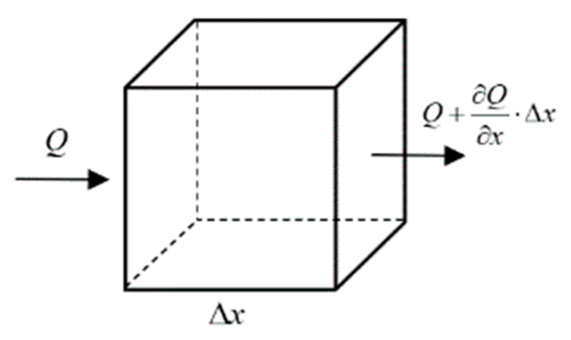
Due to the Brownian motion of molecules in static water, the particles in water move irregularly. Diffusion of molecules is the only reason for the diffusion of pollutants in the stationary water, which also exists in all the flowing water. Fick, a German physiologist, proposed that pollutants in stationary water are transported in a certain direction (through per unit area at per unit time), in direct proportion to the concentration gradient, on account of the effect of molecular diffusion, as shown in Figure 1.
Supposing that is the diffusion solute concentration located at and time , is the rate of change of diffusion mass to time in this control volume, and is the quantity of change. is the diffusion mass flux entering the surface of per unit time, is the flux out of the side. According to the conservation of mass, the difference between the mass of the incoming pollutants, per unit time, and the mass of the outgoing pollutants, per unit time, is the rate of change of the pollutant mass over time, that is:
From Fick’s diffusion law , the one-dimensional molecular diffusion equation can be obtained as follows:
By extending the one-dimension molecular diffusion equation to the two-dimension equation, can be obtained by combining Fick’s diffusion law with , and the two-dimension molecular diffusion equation can be calculated using the planar rectangular coordinate system as follows:
where , , and denote diffusivity in the x-axis and y-axis directions, respectively. Adopting a more general derivation for the convenience of later use, when meet the initial time condition , and are the boundary conditions. Using the Leibniz equation, assuming , the Equation (6) can be obtained as follows:
Only when the two parentheses are equal to zero, respectively, can the above equation be identical to zero, thus and can calculated.
In terms of , that is:
where is the mass of the pollutant. and are the position coordinates relative to the source points, and is the time.
Because the normal distribution of concentration in this paper only considers the diffusion of pollutants in water, caused by the movement of water molecules, that is, , so
where is the molecular diffusion coefficient, which is related to the characteristics of the medium, and the substance itself, as well as temperature and pressure.
2.2.2. Gaussian Plume Model
The Gaussian plume model has been extensively applied in air pollution control. Since the distribution of pollutants in water is similar to the diffusion in the atmosphere, and is a normal distribution solution to the infinite space diffusion equation, the Gaussian plume model can be used to simulate the diffusion of pollutants in water. The two-dimensional mathematical model of continuous point source diffusion is:
where and are the horizontal and vertical coordinates relative to the pollution source. stands for source strength. is the rate of emission of the pollutant source. is the degree of influence of point by the pollution source at time , with the unit of . The y-axis is defined as the diffusion direction. and are the standard deviations in the horizontal and vertical directions, respectively. That is, the diffusion coefficients in the x-axis and y-axis.
2.2.3. Forecast and Detection Update
Generally, the greater the information concentration in the task area, the higher the search reward. In order to quantify the characteristics of the task area, the information concentration map is used to describe the distribution of environmental pollutant concentrations in the water area. Predict the diffusion of pollutants according to Section 2.2.1 and Section 2.2.2 to obtain the final predicted pollutant concentration distribution . Because the pollutants change little after a long time of diffusion, it is assumed that the pollutants after the final prediction will not diffuse, that is, they will not change with time. The task area is transformed into a standard rectangle and discretized into square grids. Each grid is assigned a value, which is the pollutant information concentration in any area, after the water environment is discretized. The initial pollutant information concentration at time can be defined as follows:
where and , respectively, represent the location coordinates of the grid.
The probability that the USV will detect the pollutant concentration in any grid, at time , can be defined as , where is the abscissa and is the coordinate of any grid. According to Equation (3), the detection probability of the sensor of USV to any grid, at time , can be obtained. The distance between the USV and the grid is defined as follows:
The Bayesian update rule based on predicted information concentration and sensor detection probability is:
where and represents the updated information concentration.
3. Algorithm Principle
3.1. Voronoi Diagram Region Division
A Voronoi diagram, as a visual segmentation method, has been extensively used in computer geometry, image processing, geography, meteorology, artificial intelligence, and other domains. In this paper, the Voronoi diagram method is responsible for dividing the entire task water environments and assigning them to each USV. Each USV works independently in its own area without collision between other USVs. Therefore, the complicated problem of cooperative search coverage of multiple USVs is simplified to the problem of regional search coverage of multiple single-USV, and the search efficiency is improved. It is thought that there are USVs in the whole task area , and the positions are . According to Voronoi diagram, sub areas of each USV can be defined as follows:
The partitioned subareas are always close to the corresponding USV, and the subareas in Equation (14) are not equal in size. Therefore, the greedy strategy is used to adjust the position of the USV, as shown in Equation (15), making the subareas equal in area.
where is the feedback gain. and are the area sizes corresponding to and , respectively. is the unit vector. When the subarea size of USV is larger than that of USV , USV moves closer to the USV and expands the subarea, until the subarea is equal in size.
3.2. Model Predictive Control (MPC)
3.2.1. Traditional Model Predictive Control
Traditional Model Predictive Control is a model-based closed-loop optimization control strategy, which has been extensively used because of its low demand on model precision, strong processing ability of constraints, and can be optimized online, with good dynamic performance and robustness. Where the water environments to be searched are unknown, the MPC can be used to plan the search track of the USVs online. The search reward in the rolling time domain and the range can be taken as the optimization index, which optimizes the tracking of all USVs. On account of the sensor detection probability and information concentration map, the search reward in the time domain is defined as follows:
By optimizing the search reward , the optimal control input of each step, in rolling time domain , can be obtained. Based on the optimal control input, only the status variables of the next step can be updated, thus ensuring that each USV always moves in the direction with the optimal search reward, until the task ends.
3.2.2. Model Predictive Control with Future Reward
However, when using the traditional MPC to solve this problem, it can only predict the index of step in the time domain for a rolling optimization, which leads to poor global optimization results and falls into a local optimal solution easily. Therefore, in order to improve the overall optimization performance, this paper proposed an MPC method with a future reward, using a Voronoi diagram to partition the mass center of pollutants, and the position of USVs in the area, to establish the future reward, with the weighted sum of the two indexes taken as the total optimization reward. At time , the mass of pollutants in each region, after being divided by the Voronoi diagram, is as follows:
where represents the proportion of water environment. The regional centroid coordinates according to Equation (17) are defined as follows:
where and are the horizontal and vertical coordinates of the pollutant concentration diffusion center in the subarea of the Voronoi diagram of the USV . Even if the current centroid coordinate is outside the pollutants when the position of the USV changes, the information concentration map will be updated, and the position of the centroid will also change. According to the motion constraints of the USV, using the position of each USV and its regional centroid , the future performance index can be defined as follows:
where is the coefficient.
Because the two performance indicators have different orders of magnitude, they need to be normalized, respectively. In terms of Equation (16), the normalized search reward is as follows:
where and , respectively, represent the maximum and minimum value of the search reward in the predicted time domain, during the optimization process.
According to Equation (20), the normalized future reward is as follows:
where and , respectively, represent the maximum and minimum value of future reward in the optimization process.
Therefore, the search coverage problem of multiple USVs in this paper is transformed into the minimum optimization problem under the constraints
where is the weight coefficient of the two indexes, which meets . is the irregular static obstacles and boundaries in the water environment to be searched, and is the path point of the USVs. Meanwhile, controlling the USVs with obstacles and boundaries is used to maintain a certain margin of safety , in order to effectively avoid collisions.
Based on the search reward and the future reward in the predicted time domain, the optimal control input can be obtained. By optimizing the control input of the future step , the state variable of the next USV step can be obtained. Each USV moves one step, and repeats the above steps, until the task ends.
In this paper, Algorithm 1 represents Model Predictive Control with future reward and Algorithm 2 represents Improved Salp Swarm Algorithm.
| Algorithm 1 Pseudocode of MPC with future reward |
| Input: Maximum and minimum speed of the USV, , ; Maximum and minimum acceleration of the USV, ; Maximum and minimum angular velocity of the USV, , ; Obstacle and path point, ; Rolling optimization of time domain length, ; Output: State Variables of USVs, , , , 1: for to end of task do. 2: Randomly initialize the state variables of each USV within the constraint condition. 3: Calculate the sum of total revenue indicators of all route points that can be reached by each USV in the future step, by Equations (21) and (22). 4: Use Algorithm 2 to find the acceleration and angular velocity of each USV that can optimize the overall optimization index. 5: Update the state variables of each USV in one step. 6: end for |
| Algorithm 2 Pseudocode of ISSA |
| Input: number of search agents, ; maximum iterations, ; number of salps, ; the lower bound of variable, ; the upper bound of variable, ; Cost function, and ; Output: Optimal solution 1: Initialize the salp population considering and 2: Calculate the fitness of each salp, based on 3: Find the global best salp 4: the best 5: while (end condition is not satisfied) 6: Update by Equation (26) 7: for to do 8: 10: Update the position of the leading salps by Equation (28) 11: else 12: Update the position of the follower salps by Equation (29) 13: end if 14: end for 15: amend the salps based on the upper and lower bounds of variables 16: Calculate the fitness of each new positioned salp, based on 17: Find the best 18: compare with and , replace if greater than, and do not change if less than 19: end for 20: return |
There are many ways to solve the minimum optimization problem, which can be solved by either the mathematical optimization method or the swarm intelligence optimization method [34,35,36,37]. The traditional mathematical optimization method has insufficient ability to solve the multi constraint problems. Therefore, this paper uses the Improved Salp Swarm Algorithm, which can be a more flexible and efficient way to solve this problem.
3.3. Salp Swarm Algorithm (SSA)
3.3.1. Standard Salp Swarm Algorithm
The standard Salp Swarm algorithm simulates the living habits of salps in the ocean. Salps belong to the salps family, with a transparent barrel-shaped appearance and a shape that closely resembles a jellyfish. In the deep sea, salps usually tend to appear in clusters and form a chain, as shown in Figure 2. The salps follow salp leaders towards the food source. Therefore, if the food source is substitued by a globally optimal food source, the salp chain will automatically move towards the global optimal solution.
First of all, the salp chain is divided into two groups, one is the leaders, the other is followers. The group leaders are the first salp in the chain, and the rest are the group of followers. The leaders guide the entire salp chain, with the followers following each other. Then the position of the salp is defined and all salp positions are stored in .
where the column vector of represents the position vector of individuals in the salp chain. represents the number of salps. is the dimension.
Assuming that there is a food source in the search space, as the target of the population, the position of the leaders is updated by the following equation:
where represents the position of the first leader salp in the dimension. is the position of the food source in the dimension. and are random numbers in . determines the moving step length. determines the moving direction. and represent the upper and lower boundaries, respectively.
Equation (25) indicates that the leader only updates the position relative to the food source. In order to avoid falling into a local optimal solution, coefficient is used to measure whether to continue the search.
where is the current number of iterations. is the maximum number of iterations.
In the whole optimization process, time is the number of iterations. Newton’s laws of motion are used to update the position of the follower in the salp chain:
where , is the position of the th follower salp, in the dimension.
3.3.2. Improved Salp Swarm Algorithm (ISSA)
For the SSA, when the leader of the salp chain updates its position, it will move around the source of food, and will not be restricted by the search scope, which makes it impossible for salps leader to conduct an accurate search at the extreme point in the late convergence period, and may even jump out of the extreme point. In order to solve this problem, this paper proposes an approach to introduce the reduction factor of the salp leaders. In the early stage of convergence, a large range of search is carried out to avoid falling into the local optimum. In the late stage of convergence, it is closer to the extreme point, without escaping, improving the precision of searching
where , represents the coefficient. Because the search scopes of the leaders in the early stage of convergence are not limited, they can move in the whole world. This time, the global search ability of the algorithm can be brought into full play. In the late period of convergence, the search scope is gradually reduced, getting closer to the extreme value, so it can ensure that the individual continues to search more accurately in a small range, and improves the local search ability.
For the SSA, the historical fitness of the follower salps is not considered, and the position update of the follower salps is calculated on the basis of the current position of the individual, and the position of the previous iteration, as shown in Equation (27). The historical fitness of the follower salps have little influence on their position update, so it is not better to assist the leaders in exploring food sources. Therefore, this paper proposes a method to consider the historical fitness of the follower salps, and to improve the influence of the historical optimal fitness of the follower on its position updating. Position updating of the follower salps is compared with the individual fitness of the last iteration to influence the next position motion. The position of the follower is updated as follows:
where , , and represent the fitness of the follower at the and positions, respectively. is the random number of . In the process of position updating of the follower salps in the salp chain, the individuals with better fitness can help the leader to explore and keep closer to the food sources, so as to improve the search efficiency.
Equation (23) can be solved by using the ISSA. The control input of the USV is used as the position of an individual salp, and the total reward index is used as the fitness of the salps.
Since the global optimal solution of the optimization problem is unknown, firstly, the ISSA is used to calculate the fitness of multiple randomly initialized salps under constraint conditions. Then the current position of the salps with the best fitness, is regarded as the food source to be pursued by the salp chain, and the positions of the leader and follower salps are updated. With the increase in the number of iterations, the position of food source is constantly updated during the optimization process, leading the USVs to gradually move towards the optimal direction of the reward. The greater the number of iterations, the closer to the global optimal solution.
4. Simulation Results and Discussion
The simulations are carried out using the Matlab software running on a 3.2 GHz AMD Ryzen 7 5800H CPU, 16GB of internal storage, which verify the feasibility and effectiveness of the method proposed in this paper. It is assumed that the size of the task water environments is , which is discretized into grids, on average. The initial information concentration map composed of the normal distribution of concentration, Gaussian plume model, and random exponential function distribution mentioned in Section 2.2, represents the initial time distribution of pollutants on the water surface, as shown in Figure 3. As the distribution of pollutants is influenced by the y-axis velocity of flow, the intensity of molecular motion, the temperature, and other external factors, the final predicted information concentration map is shown in Figure 4. Other parameters are defined as follows. Number of USVs , , , , , , , Step size , feedback gain , and, maximum iterations , . The average time to run an MPC with an ISSA optimization algorithm in each step, to obtain the control inputs of the next three steps, is about 2.1s. The values of each parameter remain the same, unless otherwise stated.
It is assumed that the positions of the three UAVs at the initial moment are known, and the tasks are carried out using the information concentration map, with the final projections attached. The Voronoi diagram is used to partition the entire water environments. The results are shown in Figure 5, where the random initial positions of the USVs are represented by the black pentagram. The method in this paper is used to plan the path of each USV. The simulation result is shown in Figure 6, where the obstacles and boundaries in the area are represented by the brown line. It can be seen that this method can make multiple USVs achieve full coverage of high-value regions.
The second scenario is established to further verify the feasibility and effectiveness of the method proposed in this paper. The initial information concentration map of the second scenario is shown in Figure 7. Using the presented method in Section 2.2, the final predicted information concentration map is shown in Figure 8. The task region is divided according to the Voronoi diagram, as shown in Figure 9, where the red pentagram represents the random initial positions of each USV. The planning path of each USV is carried out using the proposed method in this paper, and the simulation result is shown in Figure 10. By comparing different values of and , it can be seen that when and , the search coverage effect of high-value regions in the task area is the best. Based on the consideration of the search reward within the range of rolling optimization, the method introduces the index of future reward, so the method can better guide the USV to search the next high-value region, and improve the search efficiency effectively, generating a track with a higher search reward. Meanwhile, the USV can avoid obstacles and the boundaries of the task area effectively, and keep a certain margin of safety. Considering the impact of noise interference on the search coverage effect, when the sensors on the USVs are affected by noise, the path planning results are shown in Figure 11. It can be seen that as the sensor detection effect under the influence of noise is weakened, the USVs will search the high-value regions many times to achieve repeated coverage.
The traditional MPC is used to plan the path of each USV in the second scenario, and the simulation results are shown in Figure 12. Because only the search reward within the predicted time domain length is taken as the indicator, the planned path will cause the USVs to be trapped in local regions, failing to cover multiple high-value regions, which greatly reduces the search efficiency. Even if there is an increase in the search time, it will not be able to cover all high-value regions.
In order to verify that the ISSA proposed in this paper produces better results when solving optimization problems compared with other methods. Using the ISSA, the SSA, Particle Swarm Optimization (PSO), Ant Colony Optimization (ACO), and Math methods, in the second scenario, under the condition that the USVs have the same initial position, the path planning problem of each USV is solved, respectively. The cumulative search reward curve of each method is shown in Figure 13. It can be seen that the cumulative search reward of ISSA is 0.9, SSA is 0.83, PSO is 0.62, ACO is 0.66, and the math method is 0.65. The method proposed in this paper has the best cumulative search reward, followed by the SSA, ACO, the Math method, and the PSO, which has the lowest cumulative search reward.
In addition, the ISSA, the SSA, the PSO, the ACO, and the Math methods are used to simulate and compare 25 tests each. The results of the cumulative search rewards are shown in Figure 14. It shows that the cumulative search reward of the ISSA in 25 tests basically remains above 0.8 and is better than the other four methods in most tests.
In the second scenario, the proposed method in this paper, the MPC, the Parallel line method, and the Random method are used to plan the path of the USVs in each region, after the Voronoi diagram division. The cumulative search reward is shown in Figure 15. It can be seen that under the same search time conditions, the final cumulative search reward of the proposed method is about 0.9. The reward of the traditional MPC, the parallel line method, and the random method is about 0.68, 0.57, and 0.28, respectively. The proposed method in this paper not only achieves the maximum search reward most of the time, but also the final result is better than the other three methods. Additionally, simulation experiments were carried out in 25 tests using the above four methods, and the results of the cumulative search rewards are shown in Figure 16. It can be seen that although the Parallel line method and the Random method are better than the methods proposed in this paper, in a few tests, the methods proposed in this paper are better than the other three methods, for most tests.
5. Conclusions
In this paper, the problem of searching and covering pollutants in unknown waters is taken as an example to study the cooperative path planning of multiple USVs. By dividing the task region with a Voronoi diagram, the complex path planning problem of multiple USVs can be transformed into several simple path planning problems of single USV. Compared with the traditional MPC, the MPC with future reward can not only plan the path of the USVs online, but also has an excellent global search performance. The ISSA is used to solve the optimization problem, which has a better search reward than the SSA and other optimization methods. The simulation results show that the method proposed in this paper has high search efficiency, can effectively cover high-value regions while avoiding obstacles, and avoids the local minimum problem in traditional methods.
In this paper, the cooperative path planning of multiple USVs for search and coverage tasks mainly considers the search coverage problem of known prior information of the task area, in the unknown environment, but does not consider the search coverage of the unknown prior information. At the same time, under the external environment such as waves, ocean current, and other disturbances [38,39,40,41], the tracking control of USVs to the planned path is not considered [42,43]. Therefore, in future work, we can consider studying how to search and cover the task area without any prior information, under environmental disturbance.
Author Contributions
Conceptualization, Z.Z., P.Y. and B.Z.; Formal analysis, Z.Z., P.Y., B.Z. and J.Y.; Methodology, Z.Z., P.Y., B.Z. and J.Y.; Validation, Z.Z., P.Y. and B.Z.; Writing—original draft, B.Z.; Writing—review & editing, B.Z., Z.Z., P.Y. and Y.Z. All authors have read and agreed to the published version of the manuscript.
Funding
This work received funding from the National Natural Science Foundation of China (61903008, 51909252).
Institutional Review Board Statement
Not applicable.
Informed Consent Statement
Not applicable.
Conflicts of Interest
The authors declare no conflict of interest.
References
- Liu, Z.; Zhang, Y.; Yu, X.; Yuan, C. Unmanned Surface Vehicles: An overview of developments and challenges. Annu. Rev. Control. 2016, 41, 71–93. [Google Scholar] [CrossRef]
- Zhou, C.; Gu, S.; Wen, Y.; Du, Z.; Xiao, C.; Huang, L.; Zhu, M. The review Unmanned Surface Vehicle path planning: Based on multi-modality constraint. Ocean Eng. 2020, 200, 107043. [Google Scholar] [CrossRef]
- Wang, Z.; Liang, Y.; Gong, C.; Zhou, Y.; Zeng, C.; Zhu, S. Improved dynamic window approach for Unmanned Surface Vehicles’ local path planning considering the impact of environmental factors. Sensors 2022, 22, 5181. [Google Scholar] [CrossRef]
- Chen, C.; Chen, X.-Q.; Ma, F.; Zeng, X.-J.; Wang, J. A knowledge-free path planning approach for smart ships based on reinforcement learning. Ocean. Eng. 2019, 189, 106299. [Google Scholar] [CrossRef]
- Niu, H.L.; Ji, Z.; Savvaris, A.; Tsourdos, A. Energy efficient path planning for Unmanned Surface Vehicle in spatially-temporally variant environment. Ocean. Eng. 2020, 196, 106766. [Google Scholar] [CrossRef]
- Yan, Z.; Li, J.; Wu, Y.; Zhang, G. A real-time path planning algorithm for AUV in unknown underwater environment based on combining PSO and waypoint guidance. Sensors 2019, 19, 20. [Google Scholar] [CrossRef] [PubMed] [Green Version]
- Zhao, Y.; Han, F.; Han, D.; Peng, X.; Zhao, W. Decision-making for the autonomous navigation of USVs based on deep reinforcement learning under IALA maritime buoyage system. Ocean. Eng. 2022, 266, 112557. [Google Scholar] [CrossRef]
- Chen, Y.; Bai, G.; Zhan, Y.; Hu, X.; Liu, J. Path planning and obstacle avoiding of the USV based on improved ACO-APF hybrid algorithm with adaptive Early-Warning. IEEE Access 2021, 9, 40728–40742. [Google Scholar] [CrossRef]
- Yu, K.; Liang, X.F.; Li, M.Z.; Chen, Z.; Yao, Y.L.; Li, X.; Zhao, Z.X.; Teng, Y. USV path planning method with velocity variation and global optimisation based on AIS service platform. Ocean Eng. 2021, 236, 109560. [Google Scholar] [CrossRef]
- Yao, Y.; Cao, J.-H.; Guo, Y.; Fan, Z.; Li, B.; Xu, B.; Li, K. Adaptive coverage control for multi-USV system in complex environment with unknown obstacles. Int. J. Distrib. Sens. Netw. 2021, 17, 15501477211021525. [Google Scholar] [CrossRef]
- Ouelmokhtar, H.; Benmoussa, Y.; Benazzouz, D.; Ait-Chikh, M.A.; Lemarchand, L. Energy-based USV maritime monitoring using multi-objective evolutionary algorithms. Ocean. Eng. 2022, 253, 111182. [Google Scholar] [CrossRef]
- Wang, L.; Wang, Z.; Liu, M.; Ying, Z.; Xu, N.; Meng, Q. Full coverage path planning methods of harvesting robot with multi-objective constraints. J. Intell. Robot. Syst. 2022, 106, 1–15. [Google Scholar] [CrossRef]
- Pathmakumar, T.; Rayguru, M.; Ghanta, S.; Kalimuthu, M.; Elara, M. An optimal footprint based coverage planning for hydro blasting robots. Sensors 2021, 21, 1194. [Google Scholar] [CrossRef] [PubMed]
- Li, L.; Chen, H. UAV enhanced target-barrier coverage algorithm for wireless sensor networks based on reinforcement learning. Sensors 2022, 22, 6381. [Google Scholar] [CrossRef] [PubMed]
- Delima, P.; Pack, D. Maximizing search coverage using future path projection for cooperative multiple UAVs with limited communication ranges. In Lecture Notes in Control And Information Sciences; Springer: Berlin/Heidelberg, Germany, 2009. [Google Scholar]
- Abd Rahman, N.A.; Sahari, K.S.M.; Hamid, N.A.; Hou, Y.C. A coverage path planning approach for autonomous radiation mapping with a mobile robot. Int. J. Adv. Robot. Syst. 2022, 19, 17298806221116483. [Google Scholar] [CrossRef]
- Lin, X.; Liu, Y. Research on multi-USV cooperative search method. In Proceedings of the 2019 IEEE International Conference on Mechatronics and Automation (ICMA), Tianjin, China, 4–7 August 2019; IEEE: Piscataway, NJ, USA, 2019. [Google Scholar]
- Fang, M.; Feng, X. Research on path planning of plant protection UAV based on grid method and improved ant colony algorithm. IOP Conf. Ser. Mater. Sci. Eng. 2019, 612, 052053. [Google Scholar]
- Luo, X.; Wang, J.; Li, X. Joint grid network and improved particle swarm optimization for path planning of mobile robot. In Proceedings of the Chinese Control Conference, Chongqing, China, 28–30 May 2017; IEEE: Piscataway, NJ, USA, 2017. [Google Scholar]
- Lee, H.K.; Jeong, W.Y.; Lee, S.; Won, J. A hierarchical path planning of cleaning robot based on grid map. In Proceedings of the 2013 IEEE International Conference on Consumer Electronics (ICCE), Las Vegas, NV, USA, 11–14 January 2013; IEEE: Piscataway, NJ, USA, 2013. [Google Scholar]
- Wen, J.; Liu, S.; Lin, Y. Dynamic navigation and area assignment of multiple USVs based on multi-agent deep reinforcement learning. Sensors 2022, 22, 6942. [Google Scholar] [CrossRef]
- Li, Z.; Shi, R.; Zhang, Z. A new path planning method based on sparse A* algorithm with map segmentation. Trans. Inst. Meas. Control 2022, 44, 916–925. [Google Scholar]
- Yong, M.; Zhao, Y.; Li, Z.; Yan, X.; Bi, H.; Królczyk, G. A new coverage path planning algorithm for Unmanned Surface Mapping Vehicle based on A-star based searching. Appl. Ocean. Res. 2022, 123, 103163. [Google Scholar]
- Dutta, A.; Bhattacharya, A.; Kreidl, O.P.; Ghosh, A.; Dasgupta, P. Multi-Robot Informative Path Planning in Unknown Environments through Continuous Region Partitioning; SAGE Publications: London, UK, 2020. [Google Scholar]
- Lu, X.; Zhi, C.; Zhang, L.; Qin, Y.; Li, J.; Wang, Y. Multi-UAV regional patrol mission planning strategy. J. Electron. Inf. Technol. 2022, 44, 187–194. [Google Scholar] [CrossRef]
- Wang, B. Path planning of mobile robot based on a algorithm. In Proceedings of the 2021 IEEE International Conference on Electronic Technology, Communication and Information (ICETCI), London, UK, 27–29 May 2021; pp. 524–528. [Google Scholar]
- Guo, X.; Chen, Y.; Zhao, D.; Luo, G. A static area coverage algorithm for heterogeneous AUV group based on biological competition mechanism. Front. Bioeng. Biotechnol. 2022, 10, 1–12. [Google Scholar] [CrossRef] [PubMed]
- Tan, G.; Zhuang, J.; Zou, J.; Wan, L. Multi-type task allocation for multiple heterogeneous Unmanned Surface Vehicles (USVs) based on the self-organizing map. Appl. Ocean. Res. 2022, 126, 103262. [Google Scholar] [CrossRef]
- Niu, X.; Zhu, J.; Wu, C.Q.; Wang, S. On a clustering-based mining approach for spatially and temporally integrated traffic sub-area division. Eng. Appl. Artif. Intell. 2020, 96, 103932. [Google Scholar] [CrossRef]
- Xiao, R.; Wu, H.; Hu, L.; Hu, J. A swarm intelligence labour division approach to solving complex area coverage problems of swarm robots. Int. J. Bio-Inspired Comput. 2020, 15, 224. [Google Scholar] [CrossRef]
- Balampanis, F.; Maza, I.; Ollero, A. Area decomposition, partition and coverage with multiple remotely piloted aircraft systems operating in coastal regions. In Proceedings of the International Conference on Unmanned Aircraft Systems, Arlington, VA, USA, 7–10 June 2016; IEEE: Piscataway, NJ, USA, 2016. [Google Scholar]
- Acevedo, J.J.; Maza, I.; Ollero, A.; Arrue, B. An efficient distributed area division method for cooperative monitoring applications with multiple UAVs. Sensors 2020, 20, 3448. [Google Scholar] [CrossRef] [PubMed]
- Chen, B.; Zhou, S.; Liu, H.; Ji, X.; Zhang, Y.; Chang, W.; Xiao, Y.; Pan, X. A prediction model of online car-hailing demand based on K-means and SVR. J. Phys. Conf. Ser. 2020, 1670, 012034. [Google Scholar] [CrossRef]
- Yu, W.; Low, K.H.; Chen, L. Cooperative path planning for heterogeneous unmanned vehicles in a search-and-track mission aiming at an underwater target. IEEE Trans. Veh. Technol. 2020, 69, 6782–6787. [Google Scholar]
- Xia, G.; Han, Z.; Zhao, B.; Liu, C.; Wang, X. Global path planning for Unmanned Surface Vehicle based on improved quantum ant colony algorithm. Math. Probl. Eng. 2019, 2019, 2902170. [Google Scholar] [CrossRef]
- Zhu, X.; Yan, B.; Yue, Y. Path planning and collision avoidance in unknown environments for USVs based on an improved D* lite. Appl. Sci. 2021, 11, 7863. [Google Scholar] [CrossRef]
- Xie, S.; Wu, P.; Liu, H.; Yan, P.; Li, X.; Luo, J.; Li, Q. A novel method of Unmanned Surface Vehicle autonomous cruise. Ind. Robot. 2016, 43, 121–130. [Google Scholar] [CrossRef]
- Razmjooei, H.; Palli, G.; Janabi-Sharifi, F.; Alirezaee, S. Adaptive fast-finite-time extended state observer design for uncertain electro-hydraulic systems. Eur. J. Control. 2022, 100749. [Google Scholar] [CrossRef]
- Razmjooei, H.; Palli, G.; Abdi, E. Continuous finite-time extended state observer design for electro-hydraulic systems. J. Frankl. Inst. 2022, 359, 5036–5055. [Google Scholar] [CrossRef]
- Razmjooei, H.; Palli, G.; Nazari, M. Disturbance observer-based nonlinear feedback control for position tracking of electro-hydraulic systems in a finite time. Eur. J. Control. 2022, 67, 100659. [Google Scholar] [CrossRef]
- Razmjooei, H.; Palli, G.; Abdi, E.; Strano, S.; Terzo, M. Finite-time continuous extended state observers: Design and experimental validation on electro-hydraulic systems. Mechatronics 2022, 85, 102812. [Google Scholar] [CrossRef]
- Duan, K.; Fong, S.; Chen, C.L.P. Reinforcement learning based model-free optimized trajectory tracking strategy design for an AUV. Neurocomputing 2022, 469, 289–297. [Google Scholar] [CrossRef]
- Woo, J.; Chanwoo, Y.; Kim, N. Deep reinforcement learning-based controller for path following of an Unmanned Surface Vehicle. Ocean. Eng. 2019, 183, 155–166. [Google Scholar] [CrossRef]
Figure 1.
One dimensional Fick diffusion.

Figure 2.
Salp chain.

Figure 3.
Initial information concentration map.

Figure 4.
Final predicted information concentration map.

Figure 5.
Regional division.

Figure 6.
Path planning based on MPC with future reward.

Figure 7.
Initial information concentration map.

Figure 8.
Final predicted information concentration map.

Figure 9.
Regional division.

Figure 10.
Path planning based on MPC with future reward (a) , , (b) , , (c) , , and (d) , .

Figure 11.
Path planning under the influence of noise.

Figure 12.
Path planning by traditional MPC (a) Search time 500 s and (b) Search time 1000 s.

Figure 13.
Cumulative search reward under different optimization methods.

Figure 14.
Cumulative detection reward by different algorithms in 25 tests.

Figure 15.
Cumulative search reward under different methods.

Figure 16.
Cumulative search reward by different methods in 25 tests.

Disclaimer/Publisher’s Note: The statements, opinions and data contained in all publications are solely those of the individual author(s) and contributor(s) and not of MDPI and/or the editor(s). MDPI and/or the editor(s) disclaim responsibility for any injury to people or property resulting from any ideas, methods, instructions or products referred to in the content. |
© 2022 by the authors. Licensee MDPI, Basel, Switzerland. This article is an open access article distributed under the terms and conditions of the Creative Commons Attribution (CC BY) license (https://creativecommons.org/licenses/by/4.0/).
Share and Cite
MDPI and ACS Style
Zhao, Z.; Zhu, B.; Zhou, Y.; Yao, P.; Yu, J. Cooperative Path Planning of Multiple Unmanned Surface Vehicles for Search and Coverage Task. Drones 2023, 7, 21. https://doi.org/10.3390/drones7010021
AMA Style
Zhao Z, Zhu B, Zhou Y, Yao P, Yu J. Cooperative Path Planning of Multiple Unmanned Surface Vehicles for Search and Coverage Task. Drones. 2023; 7(1):21. https://doi.org/10.3390/drones7010021
Chicago/Turabian StyleZhao, Zhiyao, Bin Zhu, Yan Zhou, Peng Yao, and Jiabin Yu. 2023. "Cooperative Path Planning of Multiple Unmanned Surface Vehicles for Search and Coverage Task" Drones 7, no. 1: 21. https://doi.org/10.3390/drones7010021