Drought Vulnerability in the United States: An Integrated Assessment


Center for Complex Hydrosystems Research, Department of Civil, Construction and Environmental Engineering, The University of Alabama, 1030 Cyber Hall, Box 870205, Tuscaloosa, AL 35487-0205, USA
*
Author to whom correspondence should be addressed.
Water 2020, 12(7), 2033; https://doi.org/10.3390/w12072033
Submission received: 30 June 2020
/
Revised: 14 July 2020
/
Accepted: 15 July 2020
/
Published: 17 July 2020
(This article belongs to the Special Issue Global Changes in Drought Frequency and Severity)
Abstract
:Droughts are among the costliest natural hazards in the U.S. and globally. The severity of the hazard is closely related to a region’s ability to cope and recover from the event, an ability that depends on the region’s sensitivity and adaptive capacity. Here, the vulnerability to drought of each state within the contiguous U.S. is assessed as a function of exposure, sensitivity, and adaptive capacity, using socio-economic, climatic, and environmental indicators. The division of vulnerability into three sub-indices allows for an assessment of the driver(s) of vulnerability of a state and as such provides a foundation for drought mitigation and planning efforts. In addition, a probabilistic approach is used to investigate the sensitivity of vulnerability to the weighting scheme of indicators. The resulting geographic distribution of relative vulnerability of the states is partially a reflection of their heterogeneous climates but also highlights the importance of sustainable adaptation of the local economy to water availability in order to reduce sensitivity and to limit the impact of drought. As such, the study at hand offers insights to local and regional planners on how to effectively distribute funds and plan accordingly in order to reduce state-level drought vulnerability today and in the future.
1. Introduction
Drought is one of the costliest natural disasters in the United States and globally [1,2,3], bringing famine and death to thousands of people globally every year [3]. Although deaths in the U.S. typically are not directly linked to drought as strongly as in developing countries [3], the impact of the drought is felt from the personal level, such as small-scale farmers having to kill off livestock following lack of drinking water or feed or having to abandon a family farm due to lack of income as a consequence of the impact the drought has on the land, to the regional scale, where drought can lead to economic slowdown, environmental degradation, and additional natural hazards in the form of wildfires [4]. Droughts occur naturally but are expected to change in frequency and severity under climate change [4,5,6,7,8]. The American Meteorological Society [9] classifies drought into four categories: meteorological, following shortages of precipitation; agricultural, as soil moisture levels decrease; hydrological, linked to decreased runoff; and socioeconomic drought, when water availability fails to meet societal needs. The first three drought types typically have a cascading effect, as shortages of precipitation lead to decreased soil moisture, which is followed by decreased runoff. The timing of the onset of socio-economic drought varies, depending on the drought vulnerability of the region.
Although numerous studies have estimated different aspects of vulnerability to more visually damaging hazards in the U.S., such as tornadoes [10,11,12], hurricanes [13,14], and floods [15,16,17,18,19], there is not yet any comprehensive assessment of drought vulnerability in the U.S.
This study aims to assess the relative drought vulnerability of each state within the contiguous U.S. Despite the significant impact that drought has on the nation, there is no comprehensive national-scale assessment of drought vulnerability in the U.S. Due to the sheer size of the U.S., the country has several different climate regimes with different aridity levels, but vulnerability is not linked to physical water scarcity alone—rather, it is the result of the combination of different parameters reflecting the system’s susceptibility to harm and ability to cope with hazards, which is a function of its exposure, sensitivity, and adaptive capacity [20,21]. The exact definition and calculation of vulnerability vary, depending on the field of research [22,23,24,25,26]. Methods can be grouped into biophysical approaches, socio-economic approaches, and integrated approaches [27]. Here, an integrated assessment approach is employed, combining the attributes from the biophysical and socio-economic approaches and conceptualizing vulnerability as a function of exposure, sensitivity, and adaptive capacity [20,26,27]. This holistic approach allows for an assessment of the driver(s) of vulnerability of a state and as such provides a foundation for drought mitigation and planning efforts.
Given the mixed economy of the U.S., the country’s population is not as vulnerable to drought as that in developing countries. In less developed countries, drought can lead to famine and has detrimental effects on the livelihoods of families and entire geographical regions because a large portion of the population support themselves through subsistence farming and food distribution networks and the government support are limited. Some research also suggests that drought in developing regions often is closely intertwined with weaponized conflicts [28,29].
Due to the repeated and detrimental consequences of drought in Africa, several studies have focused on the assessment of drought-related vulnerabilities in the continent [7,30,31,32] as well as other developing regions, including the Middle East [33,34,35,36] and Latin America [37].
While national-scale assessments of physical drought patterns and intensity exist for many industrialized countries [38,39,40,41,42], integrated national-scale assessments of drought vulnerability of developed countries are few [43,44,45]. Rather, the majority of research on drought vulnerability is limited to regional studies [35,36,46,47,48,49,50], specific events [51,52,53,54,55,56], or analyses of drought impacts on certain biomes [57,58,59], animal species [60,61], and economic impacts [1,62,63]. In the U.S., an exception is the work of Padowski and Jawitz [64], which assessed the water availability and associated vulnerability in 225 U.S. cities, but even this study limits itself to physical water availability and does not consider the relative sensitivity of the system and any adaptive capacity, a limitation it shares with earlier global studies on water scarcity [65,66]. The regional studies, although valuable for the region involved, fail to see the broader picture of vulnerability that allows for comparison of relative vulnerability, which is offered by a larger-scale study such as the one undertaken here.
2. Materials and Methods
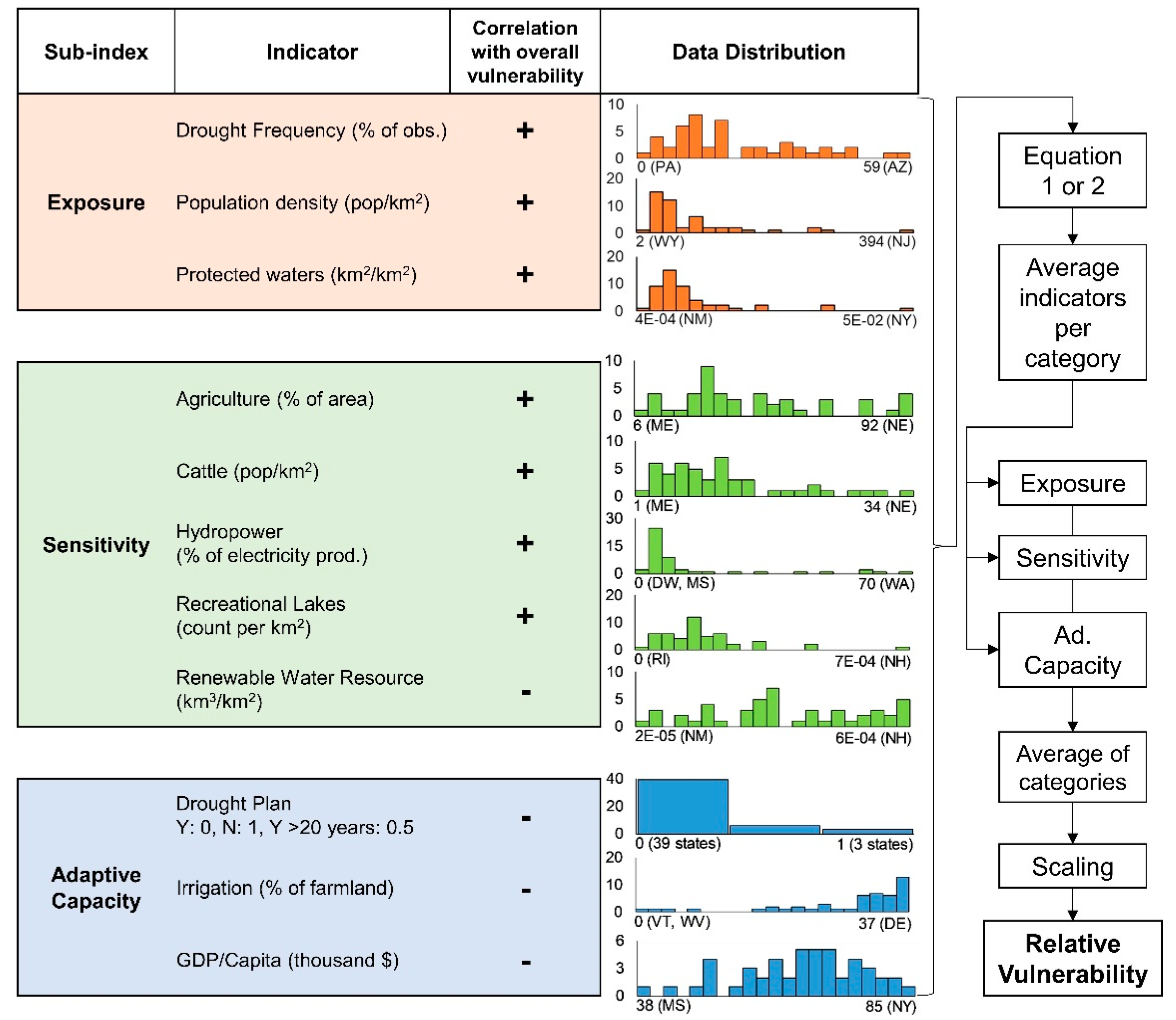
The relative vulnerability score, or Drought Vulnerability Index (DVI), can be explained as the weighted average of a set of indicators corresponding to the three categories of Exposure, Sensitivity, and Adaptive Capacity in the area of study. The main challenges in the calculation of the DVI are to (1) define an effective set of indicators that reflect the vulnerability in each drought category and state and (2) assign the proper weight to each indicator because, depending on the value of these weights, the DVI can vary significantly. To address the first challenge, the next three sections explain the indicators of each category in detail. In the Result section, first a deterministic approach where the categories Exposure, Sensitivity, and Adaptive Capacity are equally weighted is performed. Then, a probabilistic approach is applied to address the second challenge of the weight estimation.
2.1. Exposure Indicators
Three indicators are used to represent the drought exposure of a state. The first one is the drought frequency, showing how often the state is in drought. This is determined using the U.S. Drought Monitor’s full weekly record 2000–2019. The U.S. Drought Monitor’s five categories (D0–D4) are determined using a suite of drought indicators combined with subjective assessments by regional experts [67]. In the present analysis, a relatively conservative approach is taken as a state is only considered to be in drought if more than 50% of its spatial extent is in drought category D1 (Moderate Drought)–D4 (Exceptional Drought) (note that drought level D0 (Abnormally Dry) is excluded). The drought frequency is calculated as the percentage of the observations meeting the drought criteria defined above.
The second drought exposure indicator is the size of the population in the state (2019) [68]. The larger the population, the greater the exposure to the drought-associated complications and the higher the water demand, and consequently the more vulnerable the state.
The natural capital that the environment provides to the society is significant but complex to estimate [69]. Yet to conduct a full assessment of exposure and vulnerability, environmental factors need to be considered. Given the heterogeneous nature of the U.S. states, it may not be feasible to come up with universal indicators representing comparable environmental exposure, sensitivity, and/or adaptive capacity in all states. Therefore, in this study, freshwater areas actively managed for biodiversity are considered as the only environmental indicator.
The third drought exposure indicator considered in this study is the freshwater ecosystems that are adversely affected by drought through decreased water levels and changed flow regimes, increased water temperature, and deteriorating water quality [70,71]. As an indicator of the number of sensitive aquatic ecosystems exposed to drought, data on the area of freshwater streams, lakes, and wetlands under active biodiversity management were obtained from the U.S. Geological Survey and The Nature Conservancy [72,73].
2.2. Sensitivity Indicators
The sensitivity parameters are related to the geography, but also the economy, of the state, and are the characteristics that influence the likelihood of a state to experience negative impacts during drought. Here, the parameters linked to how water in the state is used are listed, together with available water resources.
The agricultural sector sustains the most direct and hardest impact during drought events. The temporal agricultural impacts range from almost instantaneous (impaired crop growth), to post-drought as drought can limit the possibilities for the planting of crops, etc., negatively affecting future revenue as well. The percentage of a state that is classified as agricultural land [74] is therefore included in the analysis.
With $66.5 billion worth of cattle produced in 2019 [75], cattle remain the most important agricultural commodity in the U.S. However, states with a large number of cattle are vulnerable to drought as the livestock requires substantial amounts of water to supply feed and drinking water through the entire production cycle [76]. Drought limits pasture yield and available drinking water, and although feed and water can be imported from other parts of the country, this leads to increased costs. Droughts therefore lead to a reduction in livestock, as seen during the 2012 drought when Oklahoma lost 23.6% (1.3 million) and Texas 16.5% (2.2 million) of their respective pre-drought cattle inventory [54]. Cattle numbers in this study are from the 2017 census [74].
Despite the recent fast development of other renewable energies, hydropower remains the leading source of renewable electricity production in the U.S. and globally [77]. The response of hydropower production to drought is slow, as is the recovery. Hydroelectricity production is hence typically not affected by flash droughts, which may be detrimental for agriculture, but long-term droughts may decrease reservoir levels substantially. This leads to decreased hydropower production, increased electricity prices (the 2012–2015 drought is estimated to have cost California residents $2 billion in increased electricity bills alone, due to decreased hydropower production in the state [78]), and increased environmental costs as the decreased hydropower production typically are compensated by increased burning of fossil fuels [78,79]. As hydropower production can vary significantly year-to-year, the average annual hydropower production 2017–2018 as a percentage of the total electricity production in the state is used in this paper [77].
Water- and lake-related recreational activities including, but not limited to, fishing, swimming, rafting, and canoeing are valuable for the local and regional economy, particularly when the lake/reservoir is located in a rural area with limited other recreational/tourism opportunities [80]. The exact economic contributions of these activities are complex to estimate due to their nonmarket nature [81]. There is limited research on the economic impact of recreational use of freshwater lakes and reservoirs, but a few studies have investigated the economic benefit of recreational freshwater fishing, including [82], who estimated the net economic value of recreational freshwater fisheries to $284 million in New York State alone and [81], that estimated the total economic impact of recreational fishing in the Sardis and Grenada reservoirs in Mississippi to $8 million annually. A decrease in water levels can limit water access and deteriorate the water quality, decreasing the income from recreational visitors. As an indicator of vulnerability linked to freshwater recreational activities, the number of recreational lakes per state is included in the analysis [83].
Renewable water resources are the sum of the water yield produced internally and transport of water in and out of the state [84]. As such, renewable water resources are complex to estimate. Here, renewable water resources per state are estimated based on [85], which used the Variable Infiltration Capacity model [86] and considered water yield produced in the basin, inflow from upstream basins, in-basin reservoir storage, trans-basin diversions, and subtracted required instream flows and downstream water supply commitments. The analysis by [85] was completed on a basin scale (HUC 4 [87]). Here, the results from [85] are generalized into five categories based on annual water yield and re-classified into yield (km3 of water per km2 area) per state. The basins are cut along the state borders, and the relative portion of renewable water in a basin is divided between the states it intersects, based on the relative areal extent of the basin in each state. The renewable water resources are closely linked to climate and drought frequency, but as it also includes factors such as in-basin storage and trans-basin diversions. The renewable water resources are heavily influenced by human interventions to the regional hydrologic cycle, interventions that serve to either increase or decrease the state’s sensitivity to drought.
2.3. Adaptive Capacity Indicators
Adaptive capacity reflects the ability of a state and its population to adapt to and recover from drought when it occurs. Indicators include both the economic strength of the state, but also state policies, and private mitigation strategies.
Whether or not a state has a drought plan is considered as a primary indicator of the state government’s awareness and concern about drought as a hazard with the potential to harm the region and strategies for adaption and mitigation. Drought plan availability, as well as the age of the plan, is collected from the National Drought Mitigation Center [68]. For this indicator, a binary system was used with a state earning a zero (0) for a drought plan, and a one (1) for the lack of a drought plan. In a secondary step, the drought plan score is increased to 0.5 if the plan is older than 20 years.
The most comprehensive protection for the impacts of drought on agriculture and forestry is the potential to irrigate the land. The amount of land being irrigated is a function of the regional climate, land use, and water laws. The area equipped for irrigation as a percentage of total farmland is therefore included as an indicator of adaptive capacity [74].
The Gross Domestic Product (GDP) per capita per state offers an indication of the economic strength of the state and its population. A strong economy makes a state less vulnerable to drought as it is more likely to have the financial muscles to mitigate and recover from the drought hazard, than a state with more limited financial means.
2.4. Drought Vulnerability Indices (DVI) and Vulnerability Classes (VC)
In those cases where the indicators’ original form is not standardized (% or per capita), the indicators are first standardized per unit area of each state (km2, U.S. Census, 2018) for size-independent comparison of the data. Next, each of the indicators is normalized separately using data from all states and considering each indicator’s maximum and minimum values. Following [31], Equation (1) is used for indicators with a positive correlation to overall vulnerability, such as population density, while Equation (2) is used for indicators with a negative correlation with overall vulnerability, such as GDP/capita.
For indicators with a positive correlation to overall vulnerability. (Equation (1))
For indicators with a negative correlation to overall vulnerability. (Equation (2))
where xi is the value of a specific indicator for the ith state, and xmin and xmax represent the maximum and minimum values of the indicator among all states. The normalized values (Z) range from 0 to 1, where zero represents the least sensitive, least exposed, and highest adaptive capacity. Setting a high adaptive capacity to zero is somewhat counterintuitive, but is required for proper comparison with the other sub-indices and calculation of the overall vulnerability. First, a deterministic assessment is conducted. The Zs are averaged per category for each state to create sub-indices (Exposure, Vulnerability, and Adaptive Capacity) and then averaged over all categories to create the DVIs showing the relative vulnerability of all states. The resulting vulnerability index is scaled according to Equation (1) and divided into five Vulnerability Classes (VCs) reflecting different relative vulnerability levels. The first group (DVI < 0.2) represents states with very low vulnerability (13 states), the second group (DVI 0.2–0.4) states with low vulnerability (19 states), the third group (DVI 0.4–0.6) states with medium vulnerability (21 states), the fourth group (DVI 0.6–0.8) states with high vulnerability (7 states), and the fifth group (DVI 0.8–1) states with very high vulnerability (3 states). An overview of the workflow as well as the distribution of the indicator data is found in Figure 1.
In the second part of the assessment, a probabilistic approach is implemented by considering the uncertainty of indicator weights. To calculate the probabilistic DVI, one thousand sets of weights are randomly generated for the indicators. Then, taking the weighted average of all normalized indicators (Zs), one thousand DVIs are calculated for each U.S. state. Multiple probability density functions (PDF) are fitted to the DVIs, and a K-S test is performed to find the best PDF for each U.S. state.
In the last step, the 0.2, 0.4, 0.6, and 0.8 quantiles ( of one thousand DVIs are used to divide the data into the five VCs of “Very Low”, “Low”, “Medium”, “High”, and “Very High” drought vulnerability. Considering the probability density function of the DVI, the probability of each VC is calculated using Equations (3)–(7).
where represents the cumulative distribution function of the ith state obtained from the PDFs.
3. Results and Discussion
3.1. Deterministic Approach
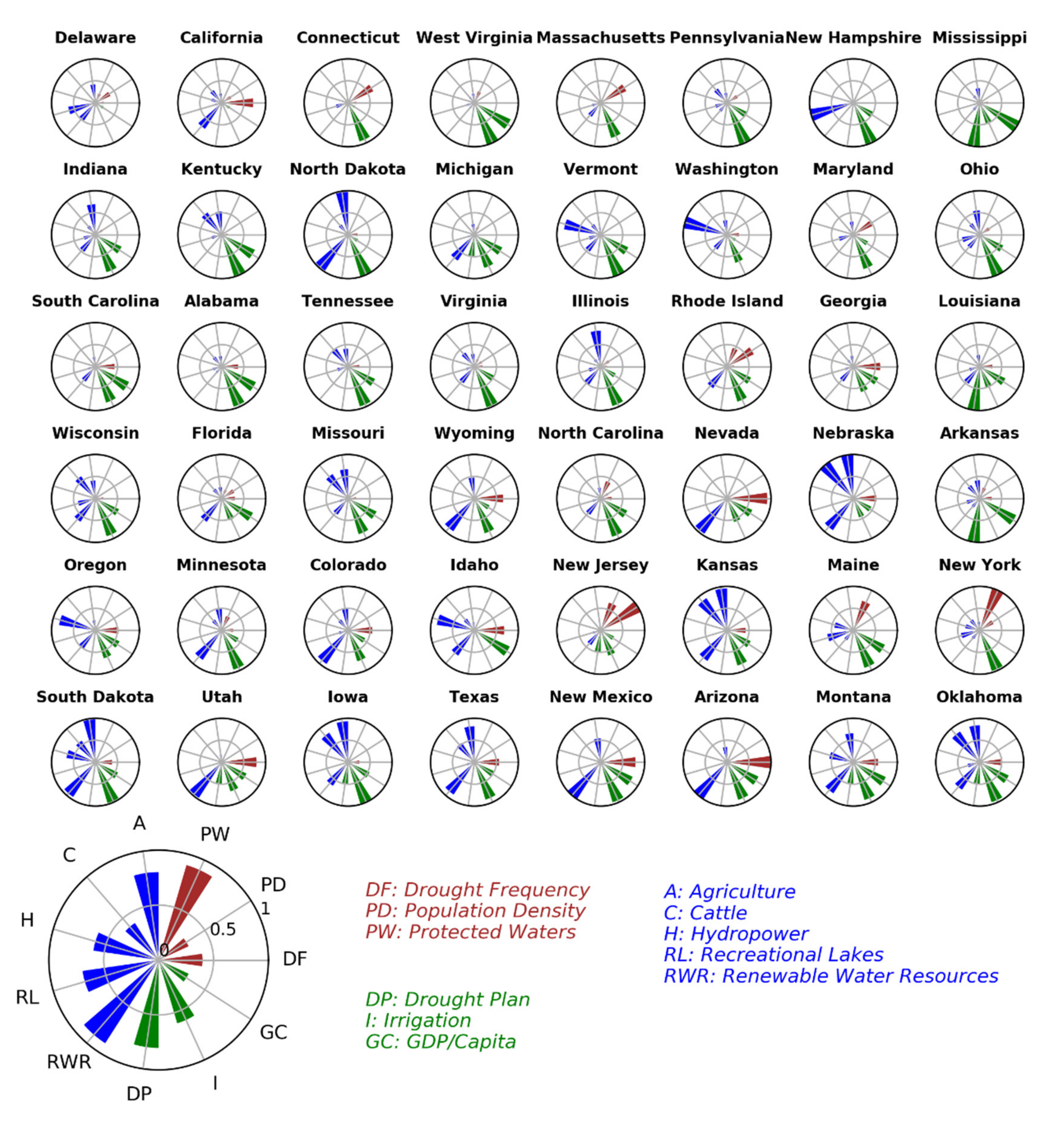
Figure 2 presents the scores of the eleven indicators for the 48 contiguous U.S. states. The template at the bottom describes the position of the indicators around the polar axes and their definitions. The indicators corresponding to the Exposure, Sensitivity, and Adaptive Capacity are shown by brown, blue, and green colors, respectively. This figure provides information for a detailed comparison of drought indicators between the U.S. states. For example, the drought vulnerability in the state of Mississippi is mostly related to the Adaptive Capacity indicators, especially drought plan and GDP/Capita. On the other hand, the state of Nebraska is vulnerable to drought due to three indicators of sensitivity, namely agriculture, cattle, and renewable water resources.
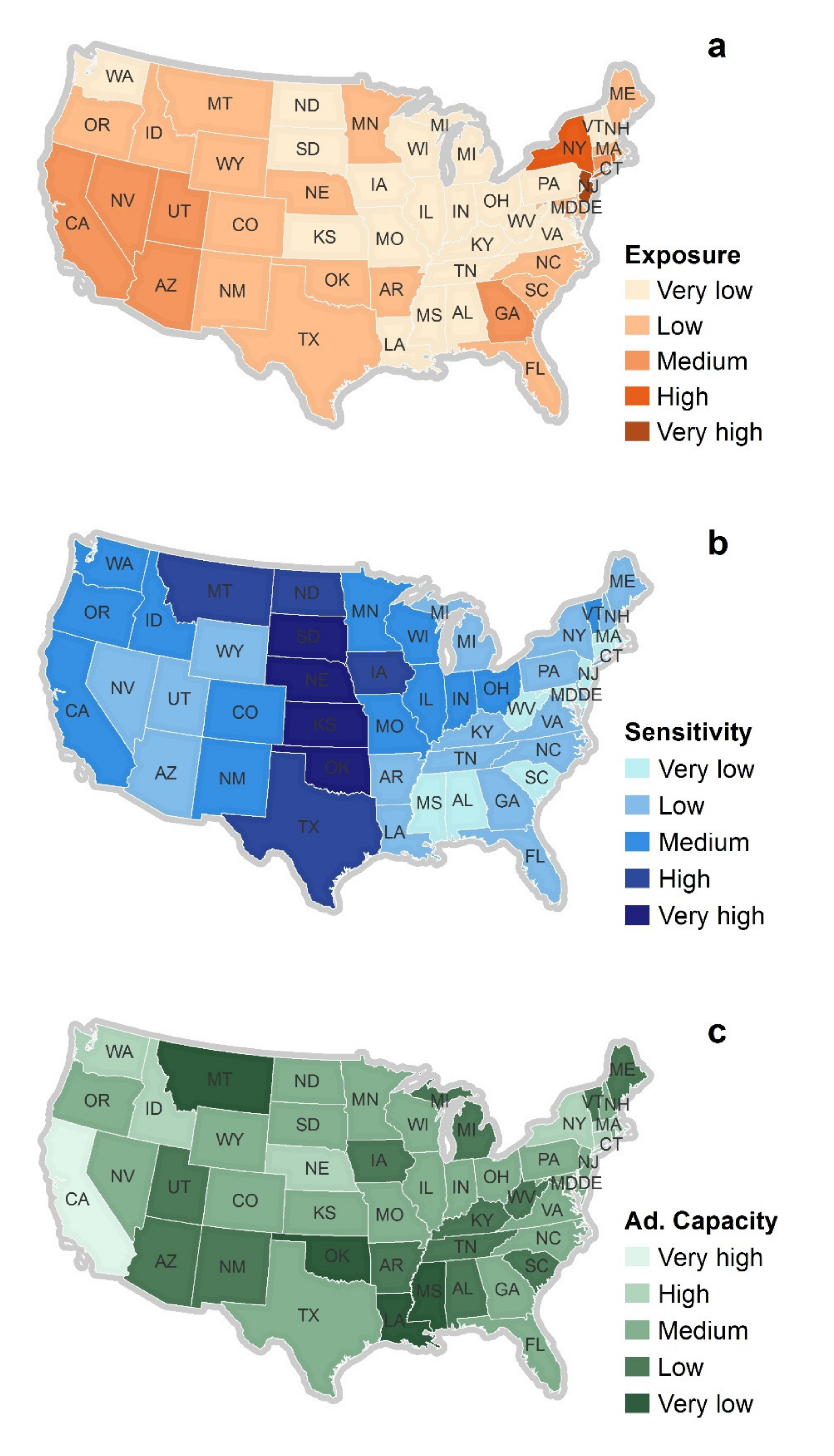
Figure 3 shows the relative exposure, sensitivity, and adaptive capacity of each state, the sub-indices that produce the overall vulnerability score. The relative vulnerability of the states in the contiguous U.S. is shown in Figure 4. The single most vulnerable state is found to be Oklahoma, while Delaware is the least vulnerable. A region that stands out as being less vulnerable than the rest of the country can be found in the northeast, extending into the eastern Mississippi Valley and the southeast (Figure 4). The humid climate in this region results in ample water resources and few droughts, leading to a generally low exposure score (Figure 3a). Sensitivity scores for this region are also below average for the country, largely due to the lack of extensive farming in these states, while the adaptive capacity scores of these states do not vary significantly compared to the rest of the states. The exemptions in this region are New Jersey, which has a very dense population, and New York, which has a very high vulnerability due to a relatively large exposure score originating from the highest percentage of protected aquatic ecosystems per unit area. Maine’s vulnerability is also ranked higher than its surrounding states. Just like New York, Maine has plenty of protected waters, as well as recreational lakes and a high dependency on hydropower.
The Southeast U.S. is slightly more drought-prone (Figure 3a) than its northern counterpart, which can be attributed to higher evapotranspiration rates. Georgia is the most drought-prone state in the Southeast U.S., but given its high adaptive capacity, its overall vulnerability is ranked as low, on a par with its neighboring states (Figure 4).
Oklahoma is ranked as the most drought-vulnerable state in the country in this study. This result is mainly attributable to limited adaptive capacity, including an outdated drought plan and limited irrigation possibilities, despite significant agricultural activities, including extensive cattle ranching (Oklahoma has 28 cattle/km2, third in the country behind Kansas (29) and Nebraska (34)). Montana is ranked as the second most vulnerable state; its vulnerability is associated mainly with a limited adaptive capacity and an above-average sensitivity originating from limited renewable water resources, extensive farming, and a significant amount of electricity being produced by hydropower.
In the Pacific Northwest, a region traditionally associated with ample precipitation, the state of Oregon stands out as being more vulnerable than its northern neighbor Washington, a difference mainly attributable to more frequent droughts in Oregon than in Washington. California, located south of Oregon, is subject to re-occurring multi-year droughts, but given its aggressive adaptation measures, it is less vulnerable than many of its neighboring states, and the second most drought-resilient state in the county.
The spectrum of vulnerability among the arid states in the southwestern part of the country spans from the “Very low” (CA) to the “High” (AZ, UT, NM) category. In this region, the physical water scarcity is profound, and the drought frequency is the highest in the country. The differences in vulnerability can hence mainly be attributed to human-related sensitivity and adaptive capacity factors. Despite being the second driest state, Nevada has adapted accordingly, to minimize dependence on limited water resources. The population density is among the lowest in the country and there are naturally few protected freshwater ecosystems, which serves to lower the overall exposure index. The sensitivity index is also low due to limited agricultural activities, hydropower, and recreational lakes, and its overall vulnerability is ranked as medium. In the same geographic cluster, Arizona, New Mexico and Utah are also found. Arizona is the single driest state in the contiguous U.S., its extremely limited water resources make it vulnerable to the exceptional water shortages associated with a drought. In New Mexico’s case, the high vulnerability score can be explained in part by extensive farming (52% of the state area is used for farming, the highest percentage in the region), in combination with limited irrigation capabilities. Utah, on the other hand, is ranked in the medium vulnerability category, a score mainly related to Utah’s limited agricultural activities in comparison to its neighboring states.
The division of the vulnerability into three sub-indices allows for analysis of the component(s) that most strongly contribute(s) to a state’s vulnerability score (Figure 3). The states with the highest exposure index are located in the Northeast (NJ and NY). Being among the least drought-prone states in the study, their high exposure scores are the fruit of their dense population and their protected aquatic ecosystems being the most extensive in the analysis. This means that droughts are rare in this region, but when they occur, a larger population of people and protected plant and animal species are at risk of being adversely affected than if the drought happened anywhere else in the contiguous U.S.
In the center of the U.S., a cluster of states emerges for which the drought sensitivity is ranked as very high (Figure 3b). In this cluster, the high sensitivity originates from their low renewable water resources in combination with extensive agricultural activities. On the other hand, low sensitivity scores across the Southeastern states are explained by ample water resources and, in comparison with other states, limited agricultural activities, hydropower, and recreational lakes.
3.2. Probabilistic Approach
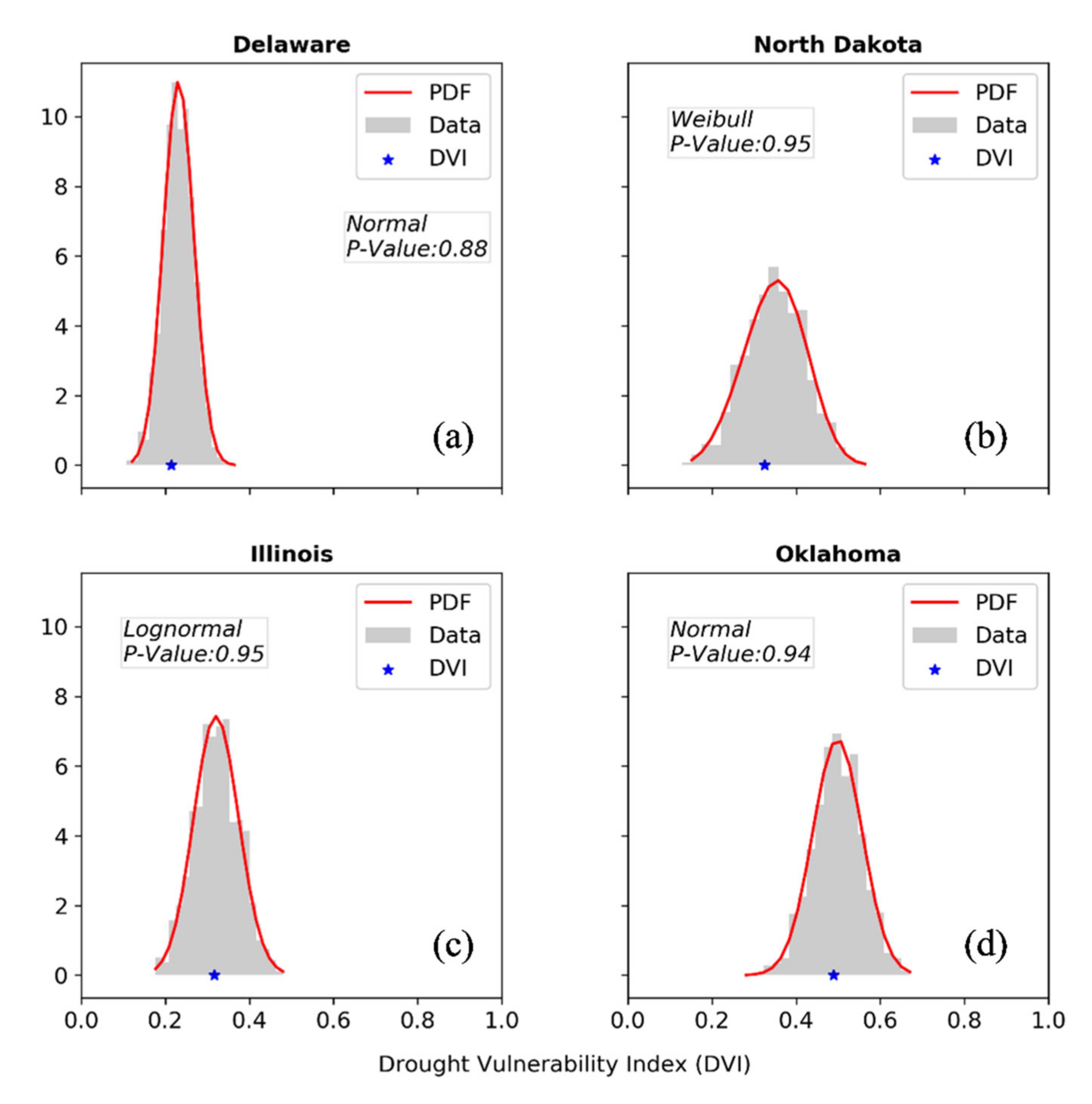
Figure 5 shows example PDFs of DVIs generated for the states of Delaware, North Dakota, Illinois, and Oklahoma. The blue point refers to the deterministic DVI, and grey bars refer to 1000 DVIs calculated from a weighted average of 11 vulnerability indicators and 1000 samples of randomly uniform weights. The shape of PDFs provides additional information about the uncertainty of DVI in each state. For example, North Dakota shows the most uncertain results despite its lower DVIs compared to Oklahoma. The highly uncertain DVI for a given state shows the high sensitivity of that state to the weights of vulnerability indicators. These states should be judiciously managed because relying on their deterministic DVI can be misleading. On the other hand, states like Delaware show very limited uncertainty and relative vulnerability.
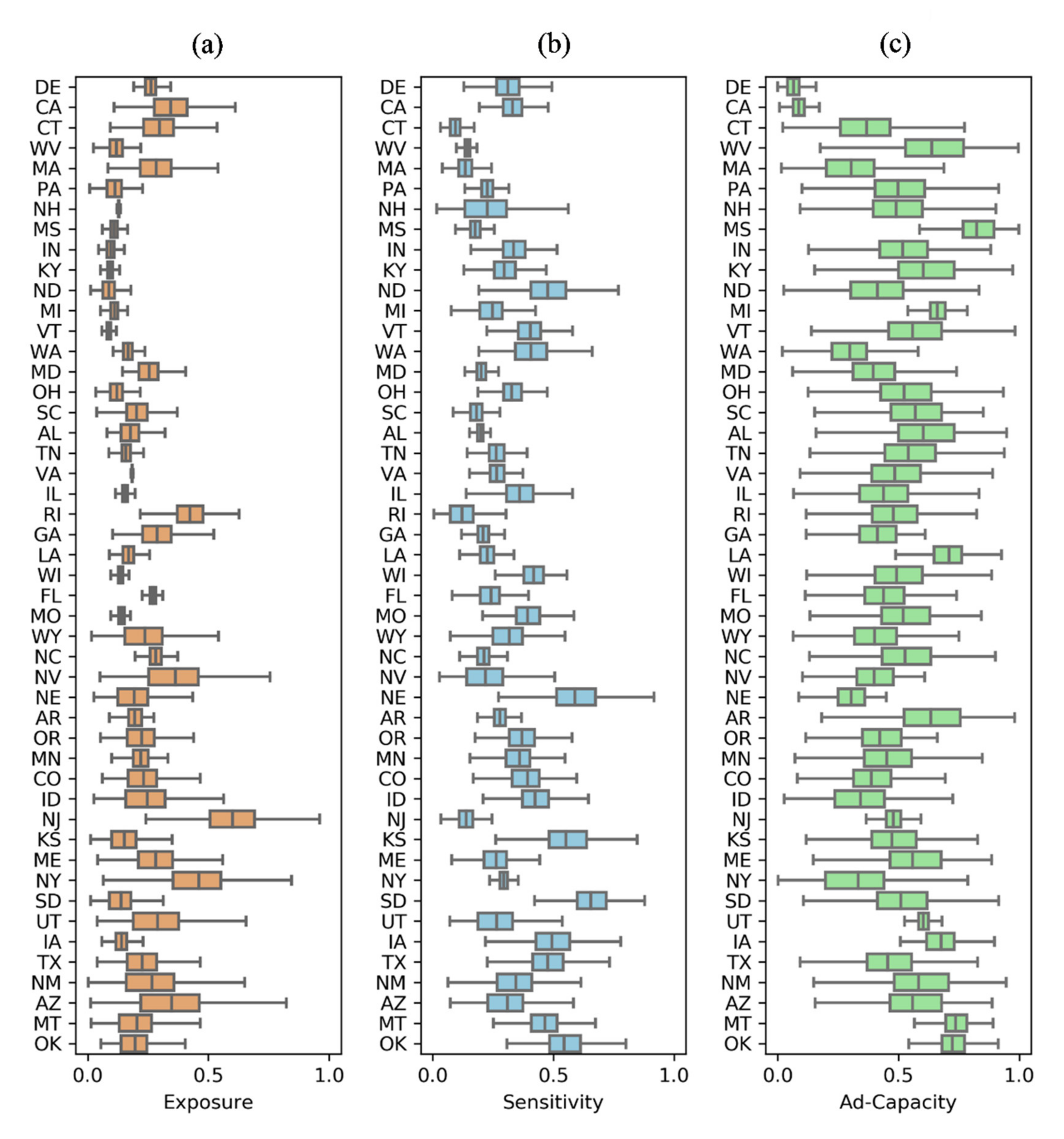
To investigate the relative vulnerability and uncertainty of the DVI components (namely Exposure, Sensitivity, and Adaptive Capacity), boxplots of distributions per category are generated (Figure 6). The boxplots show that Adaptive Capacity is the most uncertain component of vulnerability. This uncertainty is mainly attributable to the largely binary adaptive capacity indicator “Drought Plan” (Figure 1), where all but six states have the extreme values of zero (current drought plan exists) or one (no drought plan on record). Similar-looking box plots of high uncertainty also appear in the other categories, but at state level, and typically occur when a state has an extreme value for one of their indicators, the weight of which significantly changes the resulting DVI. Figure 6 also eases the state-wise comparison of DVI per category and their uncertainties. For example, a comparison between New Jersey and New York shows that both states have high exposure with large uncertainty. This can be related to their geographical location, where both states are subject to the same climatic conditions. The uncertainty of sensitivity at both states is also a small value, while the value of sensitivity is higher in New York. However, the adaptive capacity of these two states is completely different. New Jersey shows high value with a small uncertainty, but New York has low value with large uncertainty. The uncertainty of categories also provides an additional message about the relative contribution of categories compared to Figure 4. For instance, both Figure 3 and Figure 6 confirm that adaptive capacity is the main indicator explaining vulnerability in the state of Mississippi. However, looking closely, Figure 6 reveals that adaptive capacity is a highly uncertain indicator in this state, and there are several occasions in which adaptive capacity can be a small value.
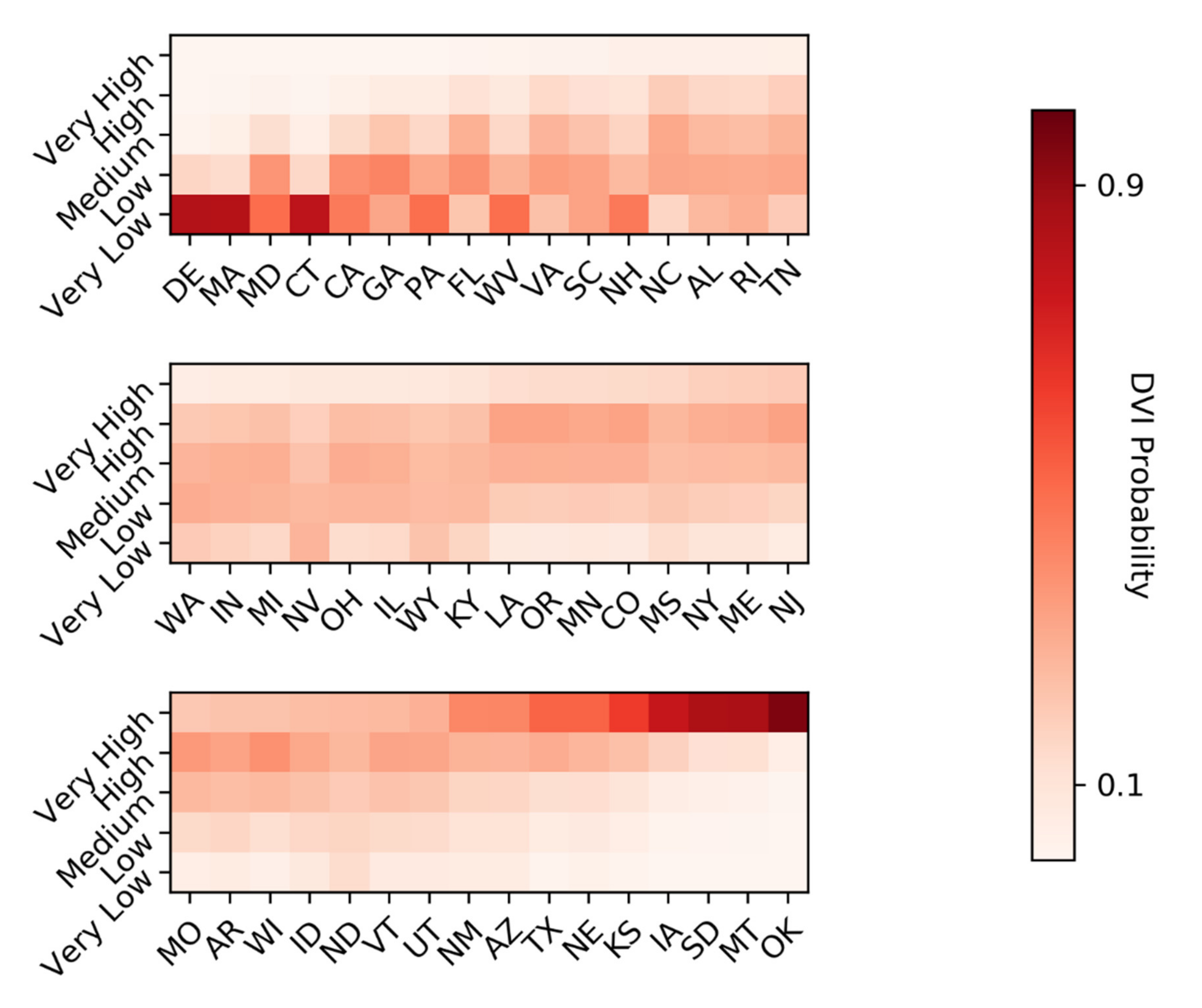
Figure 7 illustrates the probabilistic VCs for the U.S. states. The main advantage of this figure is that while it simplifies the interpretation of the vulnerability index by dividing it into five classes, it still accounts for the uncertainty of weights. The figure distinguishes states with clear VCs from those with highly uncertain VCs. For example, the states of Delaware, Massachusetts, Montana, and Oklahoma show very high certainty in their classifications. Some states, however, are more sensitive to the weights of indicators, and assigning a single VC to these states should be done with caution.
When comparing the maps in Figure 3a–c, a few geographic patterns emerge. Typically the states with medium to very high exposure scores have low, or even very low sensitivity scores. This is probably due to long-term adjustment strategies, as historically, empirical data has tended to influence regional economic development and steer it away from sectors that are not profitable in the geographical (and climatological) setting. Industrialization and modern technology have somewhat eased these natural constraints, but their historical impact is still visible.
The extent of modern-day preparedness for drought as a hazard is reflected in Figure 3c, showing adaptive capacity. This map mirrors some of the same patterns: states with medium to very high exposure scores typically have a competitive adaptive capacity score. The opposite is also true; it is among the states with the lowest exposure scores that the adaptive capacity also is lacking. This means that these states are very unlikely to be subject to a severe drought, but when they are, they have limited ability to respond to and recover from the hazard, making them vulnerable. The equal weighting of the indicators and sub-indices in this study fails to capture this vulnerability. An alternative weighting scheme could consider this and alter the results, but would introduce a different set of limitations, as the source of vulnerability is different in every state. Rather, policymakers and planners are encouraged to not limit their attention to their relative vulnerability ranking (Figure 4) but also to consider their sensitivity and adaptive capacity score (Figure 3) to find the source of their vulnerability and work on improving those areas. What is also important to consider is that the relative impact of drought varies by state. For example, a drought impacting Nebraska with its vast agricultural lands (92% of state area) could be argued to be more severe than a drought impacting a state like Alabama, which uses less than 26% of its land for agriculture; however, Alabama’s ability to cope and recover from drought is limited due to economic and policy restraints, and hence the impact on the agriculture, farmers, and the state as a whole might be more severe in Alabama.
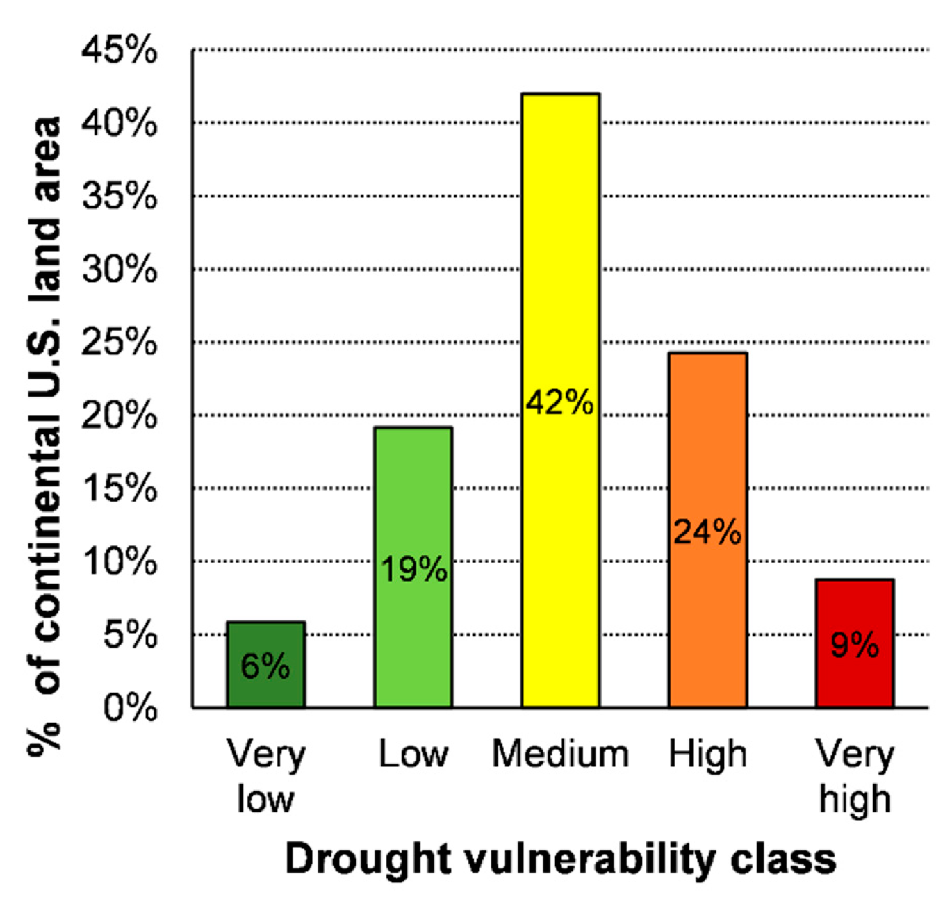
Going beyond the individual state borders, the areal percentage of contiguous U.S. found in each drought vulnerability category is shown in Figure 8. 25% of the area is in the low or very low category, 42% in the medium category, and 33% in the high or very high categories. It should be noted that the high and very high categories only contain seven and three states respectively, but these states constitute a significant portion of the contiguous U.S. As a comparison, the very low category, which covers 6% of the area, comparable to that of the highest vulnerability category, contains four states.
The study at hand gives a snapshot of current vulnerability to drought in the U.S. The indicators used show limited changes over time, but it is expected that the drought frequency and hence exposure to drought will change as a consequence of climate change. An analysis of future drought vulnerability would, apart from considering a changed exposure, also need to consider updated adaption strategies; however, such an analysis is beyond the scope of this research.
4. Conclusions
This study takes a holistic perspective on drought vulnerability in the contiguous U.S. There is no universal method for assessing vulnerability to drought or other natural hazards; therefore, the choice of indicators is directly tied to the resulting vulnerability score. In this study, the selection of indicators is limited to those where quantitative values are available at the continental-scale for all the U.S. states. Due to this limitation, the adaptive capacity may not be fully characterized with the three indicators used in this study. Therefore, to better represent the role of adaptive capacity on the drought vulnerability, future studies can specifically focus on the estimation of more quantitative continental-scale indicators of adaptive capacity. Using additional indicators, such as climate change adaptation plans and social perception of risk, can improve the overall performance of drought vulnerability analysis over the U.S. Another useful study is to specifically focus on those U.S. states with highly uncertain DVIs. In these states, the current indicators and techniques can be improved, and a more detailed analysis would be beneficial. The regional scale DVI forecast can also be carried out in states with high DVI. The access to more indicators at the regional scale provides an opportunity to perform a reliable forecast and design effective strategies for potential droughts in the near future in these states.
The vulnerability score is based on state-specific attributes as national support, such as economic compensation to farmers during drought, which is assumed to be equal throughout the country. The indicators included are chosen to represent a wide vulnerability spectrum, from water scarcity to energy and economic factors, many of which are closely intertwined with societal wellbeing. By using indicators representing different aspects of drought exposure, sensitivity, and adaptive capacity to the hazard, a drought vulnerability score is calculated, and the U.S. states are ranked according to their relative vulnerability. The states of Oklahoma, Montana, and Iowa are ranked as the most vulnerable states, while Delaware, Massachusetts, Connecticut and California are ranked as the most resilient. The geographic distribution of relative vulnerability of the states is partially a reflection of the climate of the different states, with arid states typically being more vulnerable than those with a more humid climate. However, the results also indicate the importance of the adaptation (or lack thereof) of the local economy to the climate in order to reduce sensitivity, as well as the development of adaptive capacity to limit the negative impact of drought, and offers insights to local and regional planners on how to effectively distribute funds in order to reduce state drought vulnerability today and in the future.
Author Contributions
Conceptualization, J.E. and H.M.; methodology, J.E., K.J., and H.M.; validation, J.E. and K.J.; formal analysis, J.E. and K.J.; investigation, J.E. and K.J.; writing—original draft preparation, J.E.; writing—review and editing, J.E., K.J. and H.M.; visualization, J.E. and K.J.; supervision, H.M.; funding acquisition, H.M. All authors have read and agreed to the published version of the manuscript.
Funding
This research was funded by the National Science Foundation (NSF EAR-1856054) and National Oceanic and Atmospheric Administration (NA18OAR4310319).
Conflicts of Interest
The authors declare no conflict of interest.
References
- Ding, Y.; Hayes, M.J.; Widhalm, M. Measuring economic impacts of drought: A review and discussion. Disaster Prev. Manag. Int. J. 2011, 20, 434–446. [Google Scholar] [CrossRef] [Green Version]
- Billion-Dollar Weather and Climate Disasters: Overview National Centers for Environmental Information (NCEI). Available online: https://www.ncdc.noaa.gov/billions (accessed on 30 June 2020).
- Atlas of Mortality and Economic Losses from Weather and Climate Extremes 1970–2012. Available online: https://public.wmo.int/en/resources/library/atlas–mortality–and–economic–losses–weather–and–climate–extremes–1970–2012 (accessed on 30 June 2020).
- Mukherjee, S.; Mishra, A.; Trenberth, K.E. Climate Change and Drought: A Perspective on Drought Indices. Curr. Clim. Chang. Rep. 2018, 4, 145–163. [Google Scholar] [CrossRef]
- Dai, A. Drought under global warming: A review. WIREs Clim. Chang. 2011, 2, 45–65. [Google Scholar] [CrossRef] [Green Version]
- Madadgar, S.; Moradkhani, H. Drought Analysis under Climate Change Using Copula. J. Hydrol. Eng. 2013, 18, 746–759. [Google Scholar] [CrossRef]
- Ahmadalipour, A.; Moradkhani, H.; Castelletti, A.; Magliocca, N. Future drought risk in Africa: Integrating vulnerability, climate change, and population growth. Sci. Total Environ. 2019, 622, 672–686. [Google Scholar] [CrossRef] [PubMed]
- Keellings, D.; Engström, J. The Future of Drought in the Southeastern U.S.: Projections from Downscaled CMIP5 Models. Water 2019, 11, 259. [Google Scholar] [CrossRef] [Green Version]
- Drought. Available online: https://www.ametsoc.org/index.cfm/ams/about-ams/ams-statements/statements-of-the-ams-in-force/drought/ (accessed on 30 June 2020).
- Boruff, B.J.; Easoz, J.A.; Jones, S.D.; Landry, H.R.; Mitchem, J.D.; Cutter, S.L. Tornado hazards in the United States. Clim. Res. 2003, 24, 103–117. [Google Scholar] [CrossRef] [Green Version]
- Senkbeil, J.C.; Scott, D.A.; Guinazu-Walker, P.; Rockman, M.S. Ethnic and Racial Differences in Tornado Hazard Perception, Preparedness, and Shelter Lead Time in Tuscaloosa. Prof. Geogr. 2014, 66, 610–620. [Google Scholar] [CrossRef]
- Strader, S.; Ashley, W.; Pingel, T.; Krmenec, A.J. Projected 21st century changes in tornado exposure. Clim. Chang. 2017, 141, 301–313. [Google Scholar] [CrossRef]
- Pita, G.; Pinelli, J.-P.; Gurley, K.; Mitrani-Reiser, J. State of the Art of Hurricane Vulnerability Estimation Methods: A Review. Nat. Hazards Rev. 2015, 16, 04014022. [Google Scholar] [CrossRef]
- Song, J.Y.; Alipour, A.; Moftakhari, H.R.; Moradkhani, H. Toward a more effective hurricane hazard communication. Environ. Res. Lett. 2020, 15, 064012. [Google Scholar] [CrossRef]
- Cho, S.Y.; Chang, H. Recent research approaches to urban flood vulnerability, 2006–2016. Nat. Hazards 2017, 88, 633–649. [Google Scholar] [CrossRef]
- Cutter, S.l.; Emrich, C.t.; Morath, D.p.; Dunning, C.m. Integrating social vulnerability into federal flood risk management planning. J. Flood Risk Manag. 2013, 6, 332–344. [Google Scholar] [CrossRef]
- Nasiri, H.; Yusof, M.J.M.; Ali, T.A.M. An overview to flood vulnerability assessment methods. Sustain. Water Resour. Manag. 2016, 2, 331–336. [Google Scholar] [CrossRef] [Green Version]
- Alipour, A.; Ahmadalipour, A.; Abbaszadeh, P.; Moradkhani, H. Leveraging machine learning for predicting flash flood damage in the Southeast US. Environ. Res. Lett. 2020, 15, 024011. [Google Scholar] [CrossRef]
- Khajehei, S.; Ahmadalipour, A.; Shao, W.; Moradkhani, H. A Place-based Assessment of Flash Flood Hazard and Vulnerability in the Contiguous United States. Sci. Rep. 2020, 10, 1–12. [Google Scholar] [CrossRef] [Green Version]
- IPCC. Climate Change 2001: Impacts, Adaptation, and Vulnerability: Contribution of Working Group II to the Third Assessment Report of the Intergovernmental Panel on Climate Change; McCarthy, J.J., Canziani, O.F., Leary, N.A., Dokken, D.J., White, K.S., Eds.; Cambridge University Press: Cambridge, UK, 2001; Volume 2. [Google Scholar]
- IPCC. Annex II: Glossary. In Climate Change 2014: Synthesis Report. Contribution of Working Groups I, II and III to the Fifth Assessment Report of the Intergovernmental Panel on Climate Change; Mach, K.J., Planton, S., von Stechow, C., Eds.; IPCC: Geneva, Switzerland, 2014. [Google Scholar]
- Hoogeveen, J.; Tesliuc, E.; Vakis, R.; Dercon, S. A Guide to the Analysis of Risk, Vulnerability and Vulnerable Groups; The World Bank: Washington, DC, USA, 2004. [Google Scholar]
- Adger, N. Vulnerability-ScienceDirect. Glob. Environ. Chang. 2006, 16, 268–281. [Google Scholar] [CrossRef]
- IPCC. Climate Change 2014: Impacts, Adaptation, and Vulnerability. Part A: Global and Sectoral Aspects. Contribution of Working Group II to the Fifth Assessment Report of the Intergovernmental Panel on Climate Change; Cambridge University Press: Cambridge, UK, 2014. [Google Scholar]
- Tánago, I.G.; Urquijo, J.; Blauhut, V.; Villarroya, F.; De Stefano, L. Learning from experience: A systematic review of vulnerability to drought. Nat. Hazards 2016, 80, 951–973. [Google Scholar] [CrossRef]
- Weis, S.W.M.; Agostini, V.N.; Roth, L.M.; Gilmer, B.; Schill, S.R.; Knowles, J.E.; Blyther, R. Assessing vulnerability: An integrated approach for mapping adaptive capacity, sensitivity, and exposure. Clim. Chang. 2016, 136, 615–629. [Google Scholar] [CrossRef] [Green Version]
- Singh, N.P.; Bantilan, C.; Byjesh, K. Vulnerability and policy relevance to drought in the semi-arid tropics of Asia–A retrospective analysis. Weather Clim. Extrem. 2014, 3, 54–61. [Google Scholar] [CrossRef] [Green Version]
- Opiyo, F.; Wasonga, O.; Schilling, J.; Mureithi, S. Resource–based conflicts in drought–prone Northwestern Kenya: The drivers and mitigation mechanisms. Wudpecker J. Agric. Res. 2012, 1, 442–453. [Google Scholar]
- Gleick, P.H. Water, Drought, Climate Change, and Conflict in Syria. Weather Clim. Soc. 2014, 6, 331–340. [Google Scholar] [CrossRef]
- Kamanga, T.F.; Tantanee, S.; Mwale, F.D.; Buranajarukorn, P. A multi hazard perspective in flood and drought vulnerability: Case study of Malawi. Geogr. Tech. 2020, 15, 132–144. [Google Scholar] [CrossRef]
- Ahmadalipour, A.; Moradkhani, H. Multi-dimensional assessment of drought vulnerability in Africa: 1960–2100. Sci. Total Environ. 2018, 644, 520–535. [Google Scholar] [CrossRef] [PubMed]
- Naumann, G.; Barbosa, P.; Garrote, L.; Iglesias, A.; Vogt, J. Exploring drought vulnerability in Africa: An indicator based analysis to be used in early warning systems. Hydrol. Earth Syst. Sci. 2014, 18, 1591. [Google Scholar] [CrossRef] [Green Version]
- Eklund, L.; Thompson, D. Differences in resource management affects drought vulnerability across the borders between Iraq, Syria, and Turkey. Ecol. Soc. 2017, 22. [Google Scholar] [CrossRef]
- Hameed, M.; Ahmadalipour, A.; Moradkhani, H. Drought and food security in the Middle East: An analytical framework. Agric. For. Meteorol. 2020. [Google Scholar] [CrossRef]
- Mohammad, A.H.; Jung, H.C.; Odeh, T.; Bhuiyan, C.; Hussein, H. Understanding the impact of droughts in the Yarmouk Basin, Jordan: Monitoring droughts through meteorological and hydrological drought indices. Arab. J. Geosci. 2018, 11, 103. [Google Scholar] [CrossRef] [Green Version]
- Taleb, O.; Mohammad, A.H.; Hussein, H.; Ismail, M.; Almomani, T. Over-pumping of groundwater in Irbid governorate, northern Jordan: A conceptual model to analyze the effects of urbanization and agricultural activities on groundwater levels and salinity. Environ. Earth Sci. 2019, 78, 40. [Google Scholar] [CrossRef] [Green Version]
- Ortega-Gaucin, D.; De la Cruz Bartolón, J.; Castellano Bahena, H.V. Drought Vulnerability Indices in Mexico. Water 2018, 10, 1671. [Google Scholar] [CrossRef] [Green Version]
- Kiem, A.S.; Johnson, F.; Westra, S.; van Dijk, A.; Evans, J.P.; O’Donnell, A.; Rouillard, A.; Barr, C.; Tyler, J.; Thyer, M.; et al. Natural hazards in Australia: Droughts. Clim. Chang. 2016, 139, 37–54. [Google Scholar] [CrossRef]
- Bordi, I.; Sutera, A. An analysis of drought in Italy in the last fifty years. Il Nuovo Cimento C 2002, 25, 185–206. [Google Scholar]
- Tarawneh, Q. Quantification of Drought in the Kingdom of Saudi Arabia. Int. J. Water Resour. Arid Environ. 2013, 2, 125–133. [Google Scholar]
- Karl, T.R.; Gleason, B.E.; Menne, M.J.; McMahon, J.R.; Heim, R.R., Jr.; Brewer, M.J.; Kunkel, K.E.; Arndt, D.S.; Privette, J.L.; Bates, J.J.; et al. U.S. temperature and drought: Recent anomalies and trends. Eos Trans. Am. Geophys. Union 2012, 93, 473–474. [Google Scholar] [CrossRef]
- Najac, J.; Vidal, J.-P.; Martin, E.; Franchisteguy, L.; Soubeyroux, J.-M. Changes in drought characteristics in France during the 21st century. EGU Gen. Assem. Conf. Abstr. 2010, 8975. [Google Scholar]
- Bonsal, B.R.; Wheaton, E.E.; Chipanshi, A.C.; Lin, C.; Sauchyn, D.J.; Wen, L. Drought Research in Canada: A Review. Atmosphere-Ocean 2011, 49, 303–319. [Google Scholar] [CrossRef]
- Kim, H.; Park, J.; Yoo, J.; Kim, T.-W. Assessment of drought hazard, vulnerability, and risk: A case study for administrative districts in South Korea. Assess. Drought Hazard Vulnerability Risk Case Study Adm. Dist. South Korea 2015, 9, 28–35. [Google Scholar] [CrossRef]
- Vargas, J.; Paneque, P. Challenges for the Integration of Water Resource and Drought-Risk Management in Spain. Sustainability 2019, 11, 308. [Google Scholar] [CrossRef] [Green Version]
- Wilhelmi, O.V.; Wilhite, D.A. Assessing Vulnerability to Agricultural Drought: A Nebraska Case Study. Nat. Hazards 2002, 25, 37–58. [Google Scholar] [CrossRef]
- Fontaine, M.M.; Steinemann, A.C. Assessing Vulnerability to Natural Hazards: Impact-Based Method and Application to Drought in Washington State. Nat. Hazards Rev. 2009, 10, 11–18. [Google Scholar] [CrossRef]
- Kiem, A.S.; Austin, E.K. Drought and the future of rural communities: Opportunities and challenges for climate change adaptation in regional Victoria. Glob. Environ. Chang. 2013, 23, 1307–1316. [Google Scholar] [CrossRef] [Green Version]
- Praskievicz, S. The myth of abundance: Water resources in humid regions. Water Policy 2019, 21, 1065–1080. [Google Scholar] [CrossRef]
- Preziosi, E.; Bon, A.D.; Romano, E.; Petrangeli, A.B.; Casadei, S. Vulnerability to Drought of a Complex Water Supply System. The Upper Tiber Basin Case Study (Central Italy). Water Resour. Manag. 2013, 27, 4655–4678. [Google Scholar] [CrossRef]
- Lund, J.; Medellin-Azuara, J.; Durand, J.; Stone, K. Lessons from California’s 2012–2016 Drought. J. Water Resour. Plan. Manag. 2018, 144, 04018067. [Google Scholar] [CrossRef] [Green Version]
- Horridge, M.; Madden, J.; Wittwer, G. The impact of the 2002–2003 drought on Australia. J. Policy Model. 2005, 27, 285–308. [Google Scholar] [CrossRef]
- Ciais, P.; Reichstein, M.; Viovy, N.; Granier, A.; Ogée, J.; Allard, V.; Aubinet, M.; Buchmann, N.; Bernhofer, C.; Carrara, A.; et al. Europe-wide reduction in primary productivity caused by the heat and drought in 2003. Nature 2005, 437, 529–533. [Google Scholar] [CrossRef] [PubMed]
- Rippey, B. The US drought of 2012. Weather Clim. Extrem. 2015, 10, 57–64. [Google Scholar] [CrossRef] [Green Version]
- Stah, K.; Kohn, I.; Blauhut, V.; Urquijo, J.; De Stefano, L.; Acácio, V.; Dias, S.; Stagge, J.H.; Tallaksen, L.M.; Kampragou, E.; et al. Impacts of European drought events: Insights from an international database of text-based reports. Nat. Hazards Earth Syst. Sci. 2016, 16, 801–819. [Google Scholar] [CrossRef] [Green Version]
- Ahmadi, B.; Ahmadalipour, A.; Moradkhani, H. Hydrological drought persistence and recovery over the CONUS: A multi-stage framework considering water quantity and quality. Water Res. 2019, 150, 97–110. [Google Scholar] [CrossRef]
- Allen, C.D.; Breshears, D.D. Drought-induced shift of a forest–woodland ecotone: Rapid landscape response to climate variation. Proc. Natl. Acad. Sci. 1998, 95, 14839–14842. [Google Scholar] [CrossRef] [Green Version]
- Jump, A.S.; Ruiz-Benito, P.; Greenwood, S.; Allen, C.D.; Kitzberger, T.; Fensham, R.; Martínez-Vilalta, J.; Lloret, F. Structural overshoot of tree growth with climate variability and the global spectrum of drought-induced forest dieback. Glob. Chang. Biol. 2017, 23, 3742–3757. [Google Scholar] [CrossRef]
- Zimmer, H.C.; Brodribb, T.J.; Delzon, S.; Baker, P.J. Drought avoidance and vulnerability in the Australian Araucariaceae. Tree Physiol. 2016, 36, 218–228. [Google Scholar] [CrossRef] [PubMed] [Green Version]
- Chessman, B.C. Identifying species at risk from climate change: Traits predict the drought vulnerability of freshwater fishes. Biol. Conserv. 2013, 160, 40–49. [Google Scholar] [CrossRef]
- Wilson, S.; Smith, A.C.; Naujokaitis-Lewis, I. Opposing responses to drought shape spatial population dynamics of declining grassland birds. Divers. Distrib. 2018, 24, 1687–1698. [Google Scholar] [CrossRef] [Green Version]
- Freire-González, J.; Decker, C.; Hall, J.W. The economic impacts of droughts: A framework for analysis. Ecol. Econ. 2017, 132, 196–204. [Google Scholar] [CrossRef]
- Kirby, M.; Connor, J.D.; Bark, R.H.; Qureshi, M.E.; Keyworth, S.W. The economic impact of water reductions during the Millennium Drought in the Murray-Darling Basin. Available online: https://ageconsearch.umn.edu/record/124490 (accessed on 11 July 2020).
- Padowski, J.C.; Jawitz, J.W. Water availability and vulnerability of 225 large cities in the United States. Water Resour. Res. 2012, 48. [Google Scholar] [CrossRef] [Green Version]
- Shiklomanov, I.A.; Rodda, J.C. World Water Resources at the Beginning of the Twenty-First Century; Cambridge University Press: Cambridge, UK, 2004. [Google Scholar]
- Hoekstra, A.Y.; Mekonnen, M.M.; Chapagain, A.K.; Mathews, R.E.; Richter, B.D. Global Monthly Water Scarcity: Blue Water Footprints versus Blue Water Availability. PLoS ONE 2012, 7, e32688. [Google Scholar] [CrossRef]
- Svoboda, M.; LeComte, D.; Hayes, M.; Heim, R.; Gleason, K.; Angel, J.; Rippey, B.; Tinker, R.; Palecki, M.; Stooksbury, D.; et al. THE DROUGHT MONITOR. Bull. Am. Meteorol. Soc. 2002, 83, 1181–1190. [Google Scholar] [CrossRef] [Green Version]
- Bureau, U.C. State Population Totals: 2010–2019. Available online: https://www.census.gov/data/tables/time-series/demo/popest/2010s-state-total.html (accessed on 30 June 2020).
- Crausbay, S.D.; Ramirez, A.R.; Carter, S.L.; Cross, M.S.; Hall, K.R.; Bathke, D.J.; Betancourt, J.L.; Colt, S.; Cravens, A.E.; Dalton, M.S.; et al. Defining Ecological Drought for the Twenty-First Century. Bull. Am. Meteorol. Soc. 2017, 98, 2543–2550. [Google Scholar] [CrossRef]
- Matthews, W.J.; Marsh-Matthews, E. Effects of drought on fish across axes of space, time and ecological complexity. Freshw. Biol. 2003, 48, 1232–1253. [Google Scholar] [CrossRef]
- Kovach, R.P.; Dunham, J.B.; Al-Chokhachy, R.; Snyder, C.D.; Letcher, B.H.; Young, J.A.; Beever, E.A.; Pederson, G.T.; Lynch, A.J.; Hitt, N.P.; et al. An Integrated Framework for Ecological Drought across Riverscapes of North America. BioScience 2019, 69, 418–431. [Google Scholar] [CrossRef] [Green Version]
- The Nature Conservancy TNC Lands. Available online: http://www.tnclands.tnc.org/ (accessed on 17 January 2020).
- U.S. Geological Survey Protected Areas Database of the United States (PAD-US): U.S. Geological Survey data release. Available online: https://doi.org/10.5066/P955KPLE (accessed on 17 January 2020).
- United States Department of Agriculture. Census of Agriculture 2017. United States Summary and State Data; United States Department of Agriculture: Washington, DC, USA, 2019.
- USDA Economic Research Service Annual cash receipts by commodity. Available online: https://data.ers.usda.gov/reports.aspx?ID=17832 (accessed on 8 January 2020).
- Mekonnen, M.M.; Hoekstra, A.Y. A Global Assessment of the Water Footprint of Farm Animal Products. Ecosystems 2012, 15, 401–415. [Google Scholar] [CrossRef] [Green Version]
- U.S. Energy Information Administration. Electric Power Monthly with Data for December 2018; Department of Energy: Washington, DC, USA, 2019.
- Gleick, P.H. Impacts of California’s ongoing drought: Hydroelectricity Generation; Pacific Institute: Oakland, CA, USA, 2015; p. 10. [Google Scholar]
- Christian-Smith, J.; Levy, M.C.; Gleick, P.H. Maladaptation to drought: A case report from California, USA. Sustain. Sci. 2015, 10, 491–501. [Google Scholar] [CrossRef]
- Marcouiller, D.W.; Kim, K.K.; Deller, S.C. Natural amenities, tourism and income distribution. Ann. Tour. Res. 2004, 31, 1031–1050. [Google Scholar] [CrossRef]
- Hutt, C.P.; Hunt, K.M.; Steffen, S.F.; Grado, S.C.; Miranda, L.E. Economic Values and Regional Economic Impacts of Recreational Fisheries in Mississippi Reservoirs. North Am. J. Fish. Manag. 2013, 33, 44–55. [Google Scholar] [CrossRef]
- Connelly, N.A.; Brown, T.L. Net Economic Value of the Freshwater Recreational Fisheries of New York. Trans. Am. Fish. Soc. 1991, 120, 770–775. [Google Scholar] [CrossRef]
- Food and Agriculture Organization of the United Nations. AQUASTAT–FAO’s Global Information System on Water and Agriculture, Georeferenced Database on Dams. Available online: http://www.fao.org/aquastat/en/databases/dams (accessed on 10 January 2020).
- Food and Agriculture Organization of the United Nations. AQUASTAT Main Database. Available online: http://www.fao.org/nr/water/aquastat/data/query/index.html?lang=en (accessed on 13 January 2020).
- Brown, T.; Mahat, V.; Ramirez, J.A. Adaptation to Future Water Shortages in the United States Caused by Population Growth and Climate Change. Earths Future 2019, 7, 219–234. [Google Scholar] [CrossRef] [Green Version]
- Cherkauer, K.A.; Bowling, L.C.; Lettenmaier, D.P. Variable infiltration capacity cold land process model updates. Glob. Planet. Chang. 2003, 38, 151–159. [Google Scholar] [CrossRef]
- Seaber, P.R.; Kapinos, F.P.; Knapp, G.L. Hydrologic Unit Maps; U.S. Geological Survey: Reston, VA, USA, 1987.
Figure 1.
The indicators used in the analysis, grouped into their respective sub-indices, Exposure, Sensitivity, and Adaptive Capacity. The correlation sign with the overall relative vulnerability is also noted. The distribution of the indicator data is shown in color-coded histograms, with the y-axis representing the number of states in each bin. The histograms also show the min and max value for each indicator and from what state the extreme values originate. The indicator data are then entered into Equation (1) or (2) for normalization, and the normalized data are then averaged by category, resulting in the sub-indices. In the final step, the three sub-indices are averaged and scaled to become the overall Relative Vulnerability score. An overview of the calculation procedure can be seen on the right-hand side of this figure.

Figure 2.
Contribution of the eleven drought indicators for the contiguous U.S. states. The brown, blue, and green colors refer to the indicators of exposure, sensitivity, and adaptive capacity, respectively. The template at the bottom describes the position and definition of indicators.
Figure 2.
Contribution of the eleven drought indicators for the contiguous U.S. states. The brown, blue, and green colors refer to the indicators of exposure, sensitivity, and adaptive capacity, respectively. The template at the bottom describes the position and definition of indicators.

Figure 3.
Maps giving an overview of the relative (a) exposure, (b) sensitivity, and (c) adaptive capacity of the contiguous U.S. states. It is noted that only one state (New Jersey) is in the “Very high” Exposure category.
Figure 3.
Maps giving an overview of the relative (a) exposure, (b) sensitivity, and (c) adaptive capacity of the contiguous U.S. states. It is noted that only one state (New Jersey) is in the “Very high” Exposure category.

Figure 4.
State-wise drought vulnerability across the U.S. Only three states are found in the most vulnerable category, namely Oklahoma, Montana and Iowa. Four states are identified as having very low vulnerability to drought, of which Delaware is the least vulnerable.
Figure 4.
State-wise drought vulnerability across the U.S. Only three states are found in the most vulnerable category, namely Oklahoma, Montana and Iowa. Four states are identified as having very low vulnerability to drought, of which Delaware is the least vulnerable.

Figure 5.
The probability density functions (PDFs) of Drought Vulnerability Index (DVI) (red line) for (a) Delaware, (b) North Dakota, (c) Illinois, and (d) Oklahoma states together with their deterministic DVI (blue point). The most appropriate distribution corresponding to the p-value of its K-S test is reported for each state.

Figure 6.
Distribution of DVIs per category ((a) Exposure, (b) Sensitivity, and (c) Adaptive Capacity) using the random weighted averaging method.
Figure 6.
Distribution of DVIs per category ((a) Exposure, (b) Sensitivity, and (c) Adaptive Capacity) using the random weighted averaging method.

Figure 7.
Probabilistic vulnerability classes (VCs) for the U.S. states. The color bar shows the probability that a given state fall within each class.
Figure 7.
Probabilistic vulnerability classes (VCs) for the U.S. states. The color bar shows the probability that a given state fall within each class.

Figure 8.
Areal portion of the contiguous U.S. found in each vulnerability category.

© 2020 by the authors. Licensee MDPI, Basel, Switzerland. This article is an open access article distributed under the terms and conditions of the Creative Commons Attribution (CC BY) license (http://creativecommons.org/licenses/by/4.0/).
Share and Cite
MDPI and ACS Style
Engström, J.; Jafarzadegan, K.; Moradkhani, H. Drought Vulnerability in the United States: An Integrated Assessment. Water 2020, 12, 2033. https://doi.org/10.3390/w12072033
AMA Style
Engström J, Jafarzadegan K, Moradkhani H. Drought Vulnerability in the United States: An Integrated Assessment. Water. 2020; 12(7):2033. https://doi.org/10.3390/w12072033
Chicago/Turabian StyleEngström, Johanna, Keighobad Jafarzadegan, and Hamid Moradkhani. 2020. "Drought Vulnerability in the United States: An Integrated Assessment" Water 12, no. 7: 2033. https://doi.org/10.3390/w12072033
Note that from the first issue of 2016, this journal uses article numbers instead of page numbers. See further details here.