Transfer Learning for Operator Selection: A Reinforcement Learning Approach

Abstract

In the past two decades, metaheuristic optimisation algorithms (MOAs) have been increasingly popular, particularly in logistic, science, and engineering problems. The fundamental characteristics of such algorithms are that they are dependent on a parameter or a strategy. Some online and offline strategies are employed in order to obtain optimal configurations of the algorithms. Adaptive operator selection is one of them, and it determines whether or not to update a strategy from the strategy pool during the search process. In the field of machine learning, Reinforcement Learning (RL) refers to goal-oriented algorithms, which learn from the environment how to achieve a goal. On MOAs, reinforcement learning has been utilised to control the operator selection process. However, existing research fails to show that learned information may be transferred from one problem-solving procedure to another. The primary goal of the proposed research is to determine the impact of transfer learning on RL and MOAs. As a test problem, a set union knapsack problem with 30 separate benchmark problem instances is used. The results are statistically compared in depth. The learning process, according to the findings, improved the convergence speed while significantly reducing the CPU time.

1. Introduction

Adaptive operator selection has been playing a crucial role in heuristic optimisation, especially in population-based metaheuristic approaches, including swarm intelligence algorithms. Since the early 1990s, the concept of Adaptive Operator Selection (AOS) and the methods developed for it have been widely known [1,2]. Most recently, AOS has been used with artificial bee colony (ABC) algorithms for the first time [3]. The study has been extended further with a dynamically built selection scheme with reinforcement learning to solve binary and combinatorial optimization problems [4]. The problem of operator selection becomes a sequencing problem in the sense that additional operators are added one after the other to make it easier to move solutions to more fruitful regions of the search space. Due to the randomness effect and the unknown nature of the search space, previously devised schemes may not provide the best or even a better option to respond to the current state of the problem. However, stochastic and dynamic programming-based approaches may work better. The success of an optimisation algorithm using a sequence of operators handled with stochastic processes can be seen as a Markovian Decision Process due to its nature. As a typical stochastic process and using gained experience, Q learning can help in selecting the best operator among several in a given search space under specific conditions. Many complex and difficult real-world problems, especially combinatorial ones, are thought to be easier to solve once the circumstances are effectively mapped to the best operators using experiences. The machine learning literature is filled with good examples and state of the art techniques for mapping problem states to the expected outcomes. However, since this has been done within the boundaries of a single problem domain, significant changes in data and domain will necessitate the duplication of the same process. Recent machine learning studies suggest that learning how to handle a case can be transferred across domains, and a certain level of success can be achieved using deep learning [5]. This article proposes a reinforcement learning-based transfer learning approach to aid search algorithms with adaptive operator selection schemes while transferring gained experience from one case/run/benchmark to another. Although it is widely acknowledged that deep learning approaches facilitate the use of pre-trained tools in solving new problems, shallow learning processes, particularly the use of building adaptive operator selection schemes within a dynamic and extremely unknown environment, such as metaheuristic search processes for problem solving, are less well understood. This is the first attempt, to the best of the authors’ knowledge, to apply transfer learning in building adaptive operator selection processes designed with reinforcement learning and implemented in swarm intelligence algorithms, such as the artificial bee colony algorithm.

The rest of the paper is organised as follows: Section 2 introduces the approaches on which the proposed method developed, while Section 3 details the proposed transfer learning approach. Extensive experimental results are provided in Section 4, and the article is concluded in Section 5.

2. Background and Related Work

This study brings a number of techniques together for devising an adaptive search process embedded in a swarm intelligence algorithm and enhanced with reinforcement learning. To keep the article self-contained, this section discusses briefly the necessary background followed by a review relevant to the proposed work.

2.1. Artificial Bee Colony Algorithm

The outmost optimisation framework used in this study is a swarm intelligence algorithm, which is the artificial bee colony algorithm (ABC). It is a population-based metaheuristic and evolutionary technique developed inspired by the foraging behavior of honey bees when seeking a quality food source [6]. There is a population of food positions, which refers to solution set in the ABC algorithm, and the artificial bees modify their positions over time to reach high-quality food. In order to find the optimal solution, the algorithm employs a group of agents known as honeybees. It is one of the efficient nature-inspired optimisation algorithms for solving continuous problems. Other swarm intelligence algorithms include ant colony optimisation (ACO) [7], which has been successfully used to solve discrete problems, and particle swarm optimisation (PSO) [8], which is a population-based stochastic optimisation algorithm that has been successfully used to solve continuous problems. There are three types of bees in the ABC algorithm, namely employer, onlooker, and scout bees. Employer bees are assigned to each food source in the first phase, and they use Equation (1) to try to increase the quality of the food source. The second stage involves onlooker bees attempting to enhance the most promising solutions, which are assigned probability values based on fitness function values using Equations (2) and (3). In the final step, onlooker bees turn into scout bees, who replace the non-improved food source with a new random viable solution.

$$v_i=x_i+rand(-1,1)(x_i-x_n)$$

(1)

$$p\left(x_i\right)=\frac{F\left(x_i\right)}{{\sum }_{j=1}^{N}F\left(x_j\right)}$$

(2)

$$F\left(x_i\right)=\left\{\begin{array}{cc}\frac{1}{1+f\left(x_i\right)}\hfill & f\left(x_i\right)\ge 0\hfill \\ 1+\left|f\right(x_i\left)\right|\hfill & \mathrm{otherwise}\hfill \end{array}\right.$$

(3)

where candidate, current, and neighbour solutions are represented by $v_i,x_i$, and $x_n$, respectively.

In this study, we will focus on using the ABC algorithm, which is widely used in various industries to solve a variety of problems, including combinatorial and binary problems. For the sake of brevity, further literature details have not been considered because the major goal of the proposed research is to emphasise building adaptive operator selection using one of the state-of-the-art machine learning techniques and investigate if transfer learning can be achieved in this respect.

2.2. Reinforcement Learning

Reinforcement Learning (RL) is a type of machine learning technique for solving sequential decision-making problems. In this technique, a learning agent interacts with the environment to improve its performance through trial and error [9]. As with any other learning techniques, it is all about mapping situations to behaviours in order to optimise some rewards. However, unlike other machine learning techniques, the main challenge in RL is that the learning agent has to discover by itself the best action to take in a given situation. That is, in RL, the agent learns by itself without the intervention of a human. Dynamic programming is often used in this technique to find the optimum strategy to maximise reward in a given situation. The following are some key terms that describe the fundamental parts of an RL problem: Environment (E)—the physical world in which the agent acts, States (S)—the situations of the agent (what is the agent’s current situation in a given state?), Actions (A)—the set of actions available to the agent, Reward ($R:S\times A\mapsto \mathbb{R}$)—the feedback from the environment (good or bad), Policy ($\Pi$)—a strategy to map the agent’s state to actions (it is a strategy that an agent uses in pursuit of goals), and Value (V)—the future reward that an agent will receive by taking an action in a particular state. The RL techniques can be implemented using various approaches, including Q-learning [9]. In this approach, the agent learns an optimal policy based on previous experience in the form of sample sequences of states, actions, and rewards. Therefore, each learning step consists of a state-transition tuple $(s_i,a_i,r_{i+1},s_{i+1})$, where $s_i\in S$ is the current state of the agent, $a_i\in A$ denotes the chosen action in the current state, $r_{i+1}\in R$ specifies the immediate reward received after transitioning from the current state to the next state, and $s_{i+1}\in S$ represents the next state.

There are different ways we can formulate any problem in RL mathematically; one of them is Markov Decision Process (MDP). In many applications, it is assumed that the agent is unaware of anything in the environment. However, in some other applications, it can be assumed that not everything in the environment is unknown to the agent; for example, reward calculation is considered to be part of the environment even though the agent has some knowledge of how its reward is calculated as a function of its actions and states. An MDP can be represented as a tuple $(S,A,T,\gamma ,R)$, where $S,A$, and R are defined above, $\gamma \in [0,1]$ is called the discount factor, and $T:S\times A\times S\mapsto [0,1]$ is called the probabilistic transition relation such that for a given state s and an action a, ${\sum }_{s^{\prime }\in S}T(s,a,s^{\prime })=1$. The system being modelled is Markovian if the result of an action does not depend on the previous actions and visited states (history) but only depends on the current state, i.e., $P(s_{t+1}\mid s_t,a_t,s_{t-1},a_{t-1},\dots )=P(s_{t+1}\mid s_t,a_t)=T(s_t,a_t,s_{t+1})$. This implies that the current state s gives enough information to the agent to make an optimal decision. That is, if the agent selects an action a, the probability distribution over the next states is the same as the last time the agent tried this action in the same state. Once an MDP is defined, we can define policies, optimality criteria, and value functions to compute optimal policies. Solving a given MDP means computing an optimal policy. More detailed discussion on this can be found elsewhere [10]. The RL techniques have been successfully used to train robotic and/or software agents for a variety of purposes, including games, in a variety of situations ranging from simple to complex problems [11]. In particular, Deep RL has recently been developed and made available for dealing with and solving complex, dynamic, online, and real-time problems. As part of the heuristic optimisation outlined below, RL approaches can also be employed in operator selection. It would be easier to develop more conscious adaptive selection methods that take inputs into account while selecting operators and awarding the outcomes of each operation.

2.3. Adaptive Operator Selection

Many NP-hard problems can be solved using evolutionary search techniques [12]. These are mostly stochastic optimisation algorithms that have already demonstrated their effectiveness in a variety of application domains. This is largely due to the parameters that the user can define based on the problem at hand. However, such algorithms are very sensitive to the definition of these parameters. There are no standard principles for an effective setting, so researchers from other domains rarely use those algorithms. One of the features that search algorithms with multiple alternative operators require is operator selection. In this paper, we focus on Adaptive Operator Selection (AOS) [1]. Since its introduction in the 1990s, many AOS approaches have been proposed in the literature, varying widely in various aspects such as the amount of knowledge to use from the algorithm’s previous performance and whether or not it is a good idea to use previous quality in the learning process. In practice, Credit Assignment (CA) and Operator Selection (OS) are the two components that are used during the operator selection process [13,14]. A definition based on fitness achievement over a solution is used in the CA component. OS, on the other hand, uses CA’s captured knowledge to determine the quality of each operator before estimating its likelihood. Finally, based on the probability assigned to each operator, a selection strategy is used to choose an operator for evolving a parent. All the parents in an episode are evolved using the same selection strategy. As the algorithm learns more about the landscape, it moves the solutions in a specific search direction after a number of episodes.

2.4. Transfer Learning

Transfer in reinforcement learning is a new field of study that focuses on developing strategies for transferring knowledge from a set of source tasks to a target task. When the tasks are similar, a learning algorithm can use the transferred knowledge to solve the target task and enhance performance significantly [15]. So far, traditional machine learning and deep learning algorithms have been intended to work in isolation. These algorithms have been designed to solve specific problems. Once the feature-space distribution changes, the models must be rebuilt from the scratch. Transfer learning techniques have been proposed to overcome the isolated learning paradigm, allowing acquired trained knowledge learnt for one problem to be used to address other related problems. The following three critical questions must be addressed during the transfer learning process: What needs to be transferred, when should it be transferred, and how should it be transferred? Depending on the domain, problem at hand, and data availability, various transfer learning techniques could be used [16]. This is crucial because one of the most difficult aspects of transfer learning for an RL agent running in a target problem is figuring out which elements of the target and source problems are the same and which parts are different. The majority of transfer learning research has been focused on general classical RL problems; however, the purpose of the proposed study will be on how to acquire transferable experience in operator selection through reinforcement learning.

2.5. Related Work

The performance of evolutionary algorithms, similar to that of the other meta-heuristics, is frequently linked to proper design decisions, such as crossover operator selection and other factors. The selection of variation operators that are efficient to solve the problem at hand is one of the parameters that has a significant impact on the performance of such algorithms. The control of these operators can be handled at both the structural and behavioural levels when solving the problem. At the behavioural level, adaptive operator selection refers to the process of deciding which of the available operators should be used at any given time. The adaptive operator selection technique is widely used to enhance the search power in many evolutionary algorithms, including in Multi-objective Evolutionary Algorithm [14]. In [14], the authors have proposed a bandit-based AOS method for selecting appropriate operators in an online manner. Their work proposes fitness-rate-rank, which is a credit assignment that updates the attributes using ranking rather than raw fitness progress.

The decomposition is well-known in traditional multi-objective optimisation, and the technique is used by [17]. The authors of [18] proposed the so-called multi-objective evolutionary algorithm with decomposition in 2007, which was the first time the decomposition technique was used in multi-objective optimisation. Despite the fact that these research studies have shown significant results, no state-of-the-art studies have taken into account situational information such as problem state. For example, while selecting an operator to develop new solutions, none of the above discussed approaches took into account the problem state and/or the history of past acts. In a slightly different direction, a few research studies in single-objective continuous optimisation have addressed the algorithm selection problem in an automated method. In [19], the authors proposed an initial approach to combine exploratory landscape analysis (ELA) and algorithm selection, concentrating on the BBOB test suite [20].

The work presented by [21] selects operators using fitness landscape and performance indicators without a structured learning process. The majority of AOS research in the literature is based on traditional dynamic programming approaches. There has never been a detailed investigation of a technique that uses reinforcement learning (RL) to consider the problem state, i.e. input data, when selecting operators. In [22], the authors present a Markov Decision Process model for selecting crossover operators during the evolutionary search. A Q-learning method is used to solve the given model. On the benchmark instances of Quadratic Assignment Problems, they have experimentally validated the efficacy of the proposed strategy. However, the work lacks a detailed presentation, as well as analysis and discussion. The work presented in [23] emphasises how AOS is developed with RL for a variable neighbourhood search algorithm to solve vehicle-routing problems with time window and open routes. However, not much detail is provided on how reinforcement learning is implemented throughout the article.

In a more recent work [4], the authors proposed an adaptive operator selection approach based on reinforcement learning. In their proposed method, the problem states are mapped to operators based on the success level per operation. Although these proposed techniques advance the state-of-the art on AOS based on RL, these are generally centred within the boundaries of one problem’s domain, and if major changes in data and domain occur, the same process must be replicated. As a result, new approaches for transferring learnt information from one problem-solving procedure to another are required. The proposed research addressed this problem by presenting a technique to determine the effect of transfer learning using RL and Metaheuristic optimisation algorithms, with the Adaptive Operator Selection method being used to choose between different available operators.

3. Proposed Approach for Transfer Learning with RL

It is well known that the transferability of knowledge and gained experience on how to solve problems optimally is quite limited. This is due to the uniqueness of the search spaces and the characteristics of the problem domain and data. However, transfer learning in the deep learning context has facilitated better performance, which can be investigated to see whether any particular level can be achieved. However, the problem data and set of parameters make each problem unique and distinct, making it difficult to apply gained experience from one problem to another. The aim of this research is to investigate how to achieve some degree of transferability. In this context, it is envisaged that the knowledge and experience gained through prior searches be carried out on three levels: (i) transferring experience across the runs of the same problem subject to different circumstances, but with the same configuration and settings; (ii) different problems with the same size and context; and (iii) different problems of various sizes and contexts.

The proposed research investigates if experience could be transferred between runs of the same problem.

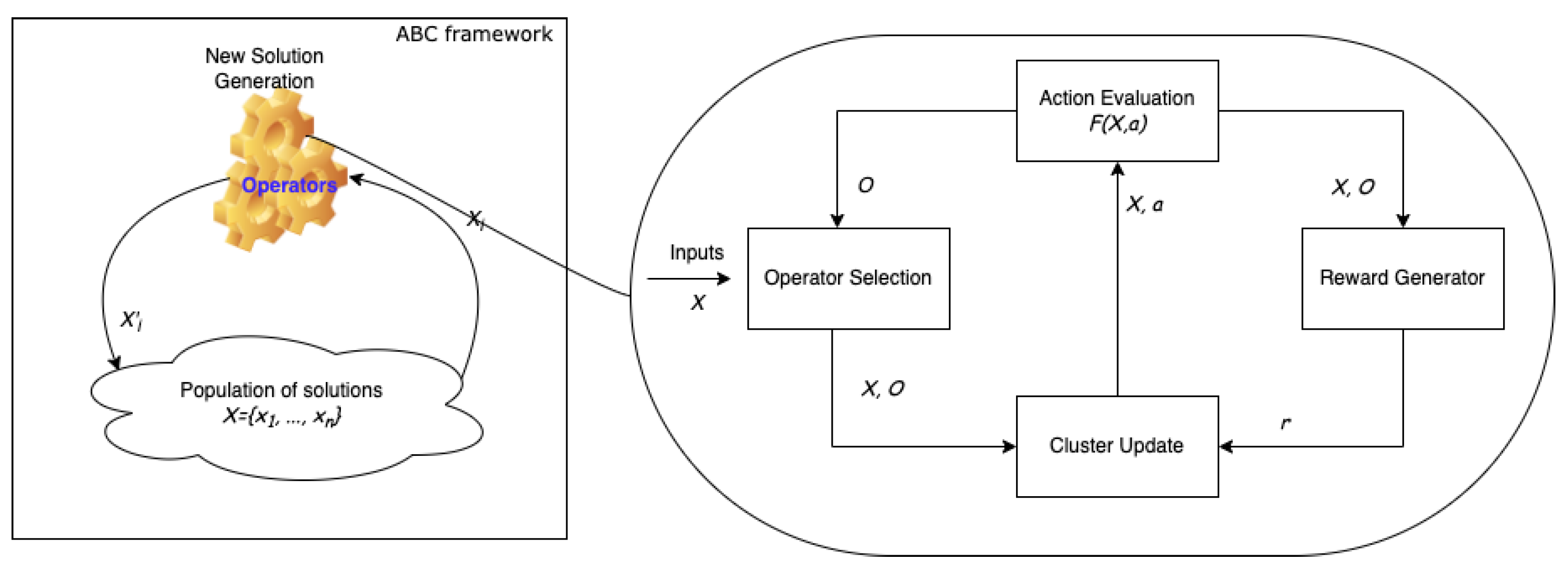
In this case, the idea of transferring learning and experience is implemented using reinforcement learning. This is achieved using a dynamic and online learning strategy to facilitate utilisation of the gained experience in different circumstances. More specifically, this turns to be the problem of dynamic operator sequencing, since an optimally selected operator to produce new solutions will be added to the list of operators selected so far. At the end of a problem-solving process, a sequence of operators will be produced via using a set of criteria such as operator selection schemes. The framework used to solve the problems whilst operator selection is learned through reinforcement learning is presented in Figure 1, where the ABC framework is depicted on the left-hand side and the details of AOS are reflected on the right-hand-side. ABC shows the interaction in between a population of solution and the new solution generator, which is detailed with the selection scheme built up with RL.

As depicted in Figure 1, a swarm intelligence algorithm (ABC works here) takes the role of the search framework, while operators are selected from a pool subject to a preferred AOS scheme. A reinforcement learning algorithm (Q learning embedded with a distance-based clustering algorithm preferred here) is placed in the search framework to work alongside the search to learn how the operators can work best subject to given circumstances. The RL algorithm continuously monitors the operator selection and the search processes to gain experience and process it accordingly to support the online operator selection scheme. The search algorithm selects an operator from the pool, applying the rule of selection scheme (here, the best Q value calculated is the rule used). Once an operator is selected, it helps to produce a new solution that is evaluated regarding whether to take it on board for the next generation or not. Depending on the success attained by the selected operator, a Q learning algorithm updates the measure for the corresponding selected operator. This is repeated until a new generation is completely built. Note that the ABC algorithm works generation-by-generation as a population-based algorithm. The complete algorithm is outlined in Algorithm 1.

Algorithm 1 General overview of RL-AOS

1: Initial Phase 2: if learning is not activated or first run then 3:     Initial credit and C cluster values 4: end if 5: Operator Selection 6: Assign probabilities 7: Choose operator using Roulette-Wheel selection 8: Operator Evaluation 9: Execute operator and get reward 10: if positive reward and learning is activated then 11:     Update cluster of operator 12:     Update operator total reward 13: end if 14: At the end of iteration 15: if learning is activated then 16:     Update credit values using Equation (5) 17: end if

We present below the above discussed concepts more formally. Let $\mathcal{X}$ be a population of solutions that makes up a bee colony handled by the ABC implemented in this study, where $\mathcal{X}=\left\{x_i\right|i=1\dots \left|\mathcal{X}\right|\}$. Each solution $x_i$ is defined as a D dimensional binary set, $x_i=\{x_{i,j}\in [0,1]|j=1\dots D\}$, and its quality of solution is measured with $F\left(x_i\right)$. The ABC is implemented uses a pool of actions $\mathcal{A}=\left\{a_k\right|k=1\dots \left|\mathcal{A}\right|\}$, where each $a_k$ is a function defined as $a_k\left(x_i\right)\stackrel{x_i}{\to }{y}_i$, where $y_i\in \mathcal{X}$. Meanwhile, a set of clusters, $\mathcal{C}=\left\{c_a\right|a=1\dots \left|\mathcal{A}\right|\}$, is defined to represent the set of actions, $\mathcal{A}$, where each cluster center is the centroid measure of the D dimensional dataset, $c_a=\{c_{a,j}|j=1\dots |D\left|\right\}$, and calculated using the following equation:

$$c_{a,j}=\frac{{\sum }_{i=0}^t{x}_{i,j}{b}_{a,i}}{{\sum }_{i=0}^t{b}_{a,i}}\forall j\in D$$

(4)

where t is the number of iterations done so far, $b_{a,i}\in [0,1]$ is a binary value indicating if the action is successful, (i.e., if the operator a helped produce a better fitness), where it take value 1 if successful and 0 otherwise. The centroids are optimised online with Q learning algorithm collecting the rewards, $r_{a,i}$, based on the fitness values, $F\left(x_i\right)$ as detailed in [4]. All $c_a$ values are initialised with 0, while random values are allocated to $Q(x,a)$. Earlier iterations impose a random selection of operators, $a\in \mathcal{A}$, whereas subsequent stages enforce the selections through fine-tuned Q values throughout the experience-gaining process. The $Q(x_i,a)$ values are updated immediately after an action is taken, (i.e., operator a is chosen and applied to $x_i$) using the following rule:

$$Q(x_i,a)=Q(x_i,a)+\beta (r_{a,i}+\gamma (E\left(y_i\right)-Q(x_i,a))$$

(5)

where $\beta$ is the learning coefficient, $\gamma$ is the discounting factor, and $E\left(y_i\right)$ is the expected Q value for the new problem’s state, i.e., a solution. The expected value is calculated with $d=|x_i-c_a|$ as the Euclidean distance between $x_i$ and $c_a$ as the current solution and the centroid for operator a, respectively. The algorithm runs repeating this procedure until a stopping criterion is satisfied. More opportunities to experience would be required to build a wide range of experience across the search space, necessitating the adoption of an exploration policy alongside the exploitation of learned cases. This study employs a $ϵ$-greedy policy to accomplish this goal. It requires randomising a value and performing a random selection if the random number is less than a $ϵ$ threshold and Q-values-based selection otherwise. More details can be found in [4,24].

The transfer learning can be adopted into a data model $\mathcal{M}\left(D\right)=\left\{m_i\left(d\right)\right|i=0\dots \left|\mathcal{M}\right|\}$, where each component of the model comprises $m_i\left(d\right)={\alpha }_i\left(d\right)⨁{\beta }_i\left(d\right)$. The model combines the terms $\alpha$ and $\beta$ with the implementation of a union operator represented by ⨁, where $\alpha$ and $\beta$ represent the experience gained previously and the experience to be gained over upcoming attempts, respectively. The model can be implemented as $m_i\left(d\right)=(1-\delta ){\alpha }_i\left(d\right)+\delta {\beta }_i\left(d\right)$, where $\delta$ is the learning coefficient that manages the contribution of previous and next experiences. For example, it switches training ON if $\delta >0$, and it switches OFF otherwise. This approach adopts transfer learning into problem solving, the data model is considered as the cluster, $\mathcal{M}\left(D\right)\stackrel{}{\leftarrow }\mathcal{C}\left(D\right)$, which is trained with solving an instance of the problem including the components as follows: $m_i\left(d\right)\stackrel{}{\leftarrow }{c}_a\left(d\right)$, $\alpha$ represents the learned components, $\beta$ is the change to be imposed from upcoming activities, and $\delta$ is to be decided if the past experience would be used.

The algorithm is set up to run once to solve a specific problem instance, with online learning switched ON to train the cluster centres and then switched OFF to repeat the experiments with the same problem instance but with new random number sequences. Since the exploration activities are pruned, this is expected to solve the problem with better or slightly better solution qualities in a far shorter period. This is the stage at which the proposed algorithm transfers previously gained experience, which is still the most common method of transfer learning.

4. Experimental Results

This section introduces experimental results of the proposed approach to handle transfer learning across different runs of the same problem instances. We demonstrate how reinforcement learning-based experience transfer assists towards solving the problem in high efficiency with respect to computational time. The experiments have been carried out in a high-performance computing cluster machine with 8 core CPU $27.2$ GB RAM and CentOS $7.9$ operating system specs.

4.1. The Problem and Datasets

This study has been conducted to demonstrate the gain/benefit of transfer learning using an adaptive operator selection scheme built with an implementation of Q learning algorithm. Both the selection scheme and the RL (i.e., Q learning) are embedded within a standard ABC algorithm equipped with three recent state-of-the-art binary operators; binABC [25], ibinABC [26], and disABC [27] to solve the set union knapsack problem (SUKP), where Q learning is implemented and integrated into the ABC algorithm to allow the agent (i.e., the ABC algorithm) to learn how to adaptively select one of these three operators.

The family of knapsack problems includes renown combinatorial optimisation problem sets used to test the efficiency and performance of problem-solving algorithms. They are known as an NP-Hard problems with respect to complexity and are very instrumental in modelling and solving real-world industrial problems. SUKP is a special form of knapsack problem, which holds NP-Hard complexity level [28]. This problem is chosen as the test-bed in this study to demonstrate the success of proposed approach. It requires a set of items to be optimally composed in subsets so as to gain the maximum benefit. Given a set of n elements, $U=\left\{u_i\right|i=1,\dots ,n\}$ with a non-negative weight set, $W=\left\{w_i\right|i=1,\dots ,n\}$ and a set of m items, $\mathcal{S}=\left\{U_j\right|j=1,\dots ,m\}$ with a profit set, $\mathcal{P}=\{p_j>0|j=1,\dots ,m\}$, a subset of $A\subseteq \mathcal{S}$ is sought to be found such that it maximises the profit subject to that the sum of the weights of selected items is not to exceed the capacity constraint, C. The formal structure of the problems is as follows:

$$maxP\left(A\right)=\sum _{j\in A}{p}_j$$

(6)

$$\mathrm{s}.\mathrm{t}.W\left(A\right)=\sum _{i\in {\bigcup }_{j\in A}{U}_j}{w}_i\le C,A\subseteq \mathcal{S}.$$

(7)

The problem is represented in real numbers and needs to be represented in binary form to enable binary operators in search algorithms such as binary ABC [3]. Following the details of the problem and the approach introduced by [29], a binary vector, $B=\left\{b_j\right|j=1,..,m\}\in \{0,1\}$, is defined to be used as the set of decision variables, where $b_j=1$ if an item is selected, $b_j=0$, otherwise. The model of the problem can be reformulated as follows:

$$maxf\left(B\right)=\sum _{j=1}^m{b}_j{p}_j$$

(8)

$$\mathrm{s}.\mathrm{t}.W\left(A_B\right)=\sum _{i\in {\bigcup }_{j\in A_B}{U}_j}{w}_i\le C.$$

(9)

The main goal is to find the best binary vector, B, which provides the subset of items with the maximum profit.

The problem instances of SUKP chosen in this study are collected from recently published literature. He et al. [30] have introduced 30 benchmarking problem instances of SUKP as tabulated in

Table 1. The SUKP benchmark instances.

${\mathbf{Set}}_{\mathbf{1}}$					${\mathbf{Set}}_{\mathbf{2}}$					${\mathbf{Set}}_{\mathbf{3}}$
ID	m	n	w	y	ID	m	n	w	y	ID	m	n	w	y
1_1	100	85	0.10	0.75	2_1	100	100	0.10	0.75	3_1	85	100	0.10	0.75
1_2	100	85	0.15	0.85	2_2	100	100	0.15	0.85	3_2	85	100	0.15	0.85
1_3	200	185	0.10	0.75	2_3	200	200	0.10	0.75	3_3	185	200	0.10	0.75
1_4	200	185	0.15	0.85	2_4	200	200	0.15	0.85	3_4	185	200	0.15	0.85
1_5	300	285	0.10	0.75	2_5	300	300	0.10	0.75	3_5	285	300	0.10	0.75
1_6	300	285	0.15	0.85	2_6	300	300	0.15	0.85	3_6	285	300	0.15	0.85
1_7	400	385	0.10	0.75	2_7	400	400	0.10	0.75	3_7	385	400	0.10	0.75
1_8	400	385	0.15	0.85	2_8	400	400	0.15	0.85	3_8	385	400	0.15	0.85
1_9	500	485	0.10	0.75	2_9	500	500	0.10	0.75	3_9	485	500	0.10	0.75
1_10	500	485	0.15	0.85	2_10	500	500	0.15	0.85	3_10	485	500	0.15	0.85

with all configuration details, where three different configurations presented varying with comparative status of m and n; (i) $m>n$, (ii) $m<n$, and (iii) $m=n$), while $w\in \{0.10,0.15\}$ and $y\in \{0.75,0.85\}$ represent the density of elements and the rate between the capacities and the sum of weights of elements, respectively. As seen, each set of problem instances includes 10 instances varying with $m,n,w$, and $y$ values. More details can be found in [30,31].

4.2. Experimental Settings

The experimental study reported in this article is conducted to demonstrate that transfer learning helps improve the efficiency of swarm intelligence algorithms in solving combinatorial optimisation problems. For this purpose, three algorithms have been set up: (i) RLABC taken from [4] is the baseline algorithm that solves the problems with ABC embedded with a Q learning-based adaptive operators selection scheme, (ii) RLABC-T extends RLABC with a static transfer learning that switches off the gain experience in upcoming runs, and (iii) RLABC-TC keeps online learning while solving new problems and executes new runs. This means $\delta =0$ for RLABC-T, while $\delta >0$ for RLABC-TC.

The parametric settings for all algorithms have been taken from previous works [3,4] rolling over the fine-tuned set of parameters accordingly. The configuration applied to all three algorithms includes the following settings: $\gamma$ is 0.3, the window size W is 25 iterations, reward is chosen as extreme (${\widehat{r}}_{i,t}$), $ϵ$ is 0.1, and $\alpha$ is 0.5. The termination criteria is used as the maximum number of iterations, which is determined as the problem size. For the algorithm parameters, the population size is 20 and maximum trial number is 100.

4.3. Results and Discussions

Table 2. Comparative results in solution quality for Set₁ benchmarks.

	RLABC				RLABC-T					RLABC-TC
	Best	Mean	Std	R	Best	Mean	Std	R	S	Best	Mean	Std	R	S
1_1	13,251	13,071.4	53.5	1	13,283	13,070.5	61.80	2	−	13,167	13,054.9	38.1	3	−
1_2	12,274	12,143.2	73.1	2	12,238	12,090.8	80.25	3	+	12,272	12,153.9	62.5	1	−
1_3	13,402	13,271.7	100.2	2	13,405	13,283	67.74	1	−	13,405	13,262.8	88.2	3	−
1_4	14,215	13,680.6	251.4	1	13,777	13,451.8	201.02	3	+	14,215	13,674.8	232.0	2	−
1_5	11,065	10,717.5	141.1	2	10,900	10,661.5	110.45	3	−	11,073	10,777.1	166.0	1	−
1_6	12,245	11,672.6	269.3	3	12,245	11,734.5	285.05	1	−	12,245	11,722.8	272.0	2	−
1_7	11,289	10,742.4	252.1	3	11,244	10,812.7	250.80	1	−	11,294	10,755.3	216.8	2	−
1_8	10,168	10,027.1	145.2	3	10,175	10,123.9	84.43	1	+	10175	10,103.8	82.4	2	+
1_9	11,427	11,188.1	140.5	3	11,490	11,196.1	134.66	2	−	11,490	11,230.6	151.2	1	−
1_10	9734	9359.3	195.2	2	9817	9475.3	154.50	1	+	10,022	9355.3	208.8	3	-
			Mean:	2.2			Mean:	1.8				Mean:	2

,

Table 3. Comparative results in solution quality for Set₂ benchmarks.

	RLABC				RLABC-T					RLABC-TC
	Best	Mean	Std	R	Best	Mean	Std	R	S	Best	Mean	Std	R	S
2_1	14,044	13,949	85.05	1	14,044	13,943.2	86.3631	2	−	14,044	13,938.5	92.7598	3	−
2_2	13,508	13,442.1	88.2756	2	13,508	13,465.9	48.2438	1	−	13,508	13,414	99.4093	3	−
2_3	12,211	11,833.3	178.218	3	12,328	11,944.3	201.902	1	−	12,328	11,845.8	212.621	2	−
2_4	12,019	11,652	163.042	2	11,821	11,627.4	201.362	3	−	12,187	11,697.1	222.437	1	−
2_5	12,646	12,535	167.639	3	12,695	12,623.3	72.6071	1	+	12,655	12,595.2	114.05	2	−
2_6	11,410	10,679.6	176.845	3	11,054	10,759.6	144.579	1	+	11,251	10,725.8	137.088	2	+
2_7	11,193	10,855.3	132.626	3	11,310	10,924.2	170.308	1	−	11,249	10,889.6	156.932	2	−
2_8	10,355	9882.63	234.754	2	10,382	9871.07	233.87	3	−	10,382	9947.37	214.996	1	−
2_9	10,770	10,647.2	65.2152	3	10,885	10,688.7	60.1216	2	+	10,885	10,694.9	73.2702	1	+
2_10	10,194	9851.07	209.2	1	10,176	9845.03	186.539	2	-	10,176	9798.8	229.578	3	-
			Mean:	2.3			Mean:	1.7				Mean:	2

and

Table 4. Comparative results in solution quality for Set₃ benchmarks.

	RLABC				RLABC-T					RLABC-TC
	Best	Mean	Std	R	Best	Mean	Std	R	S	Best	Mean	Std	R	S
3_1	12,045	11,632	191.489	3	12,020	11,697.3	148.956	1	−	12,020	11,651.9	152.747	2	−
3_2	12,369	12,205.2	149.614	1	12,369	12,101	263.167	3	−	12,369	12,196.8	201.196	2	−
3_3	13,609	13,352.2	130.039	2	13,609	13,399	99.6629	1	−	13,609	13,334.8	127.075	3	−
3_4	10,973	10,856.3	105.533	2	11,021	10,852.4	86.8795	3	−	11,298	10,859.1	140.543	1	−
3_5	11,538	11,240	169.691	3	11,538	11,308.8	210.61	1	−	11,538	11,287.8	194.904	2	−
3_6	11,377	11,077.2	189.324	1	11,377	11,017.5	178.618	2	−	11,377	10,997.4	202.552	3	+
3_7	10,181	9951.63	80.973	1	10,069	9932.27	67.0159	3	−	10,087	9946.9	76.4209	2	−
3_8	10,075	9403.8	177.593	3	10,077	9517.33	193.699	1	+	9749	9445.77	146.641	2	−
3_9	10,877	10,647.3	101.085	2	10,831	10,626.4	90.5375	3	−	10,987	10,668.8	122.98	1	−
3_10	9745	9426.57	136.45	2	10,220	9433.83	234.262	1	-	9649	9421.17	117.068	3	-
			Mean:	2			Mean:	1.9				Mean:	2.1

show comparisons among three variants in terms of solution quality. The column of best is determined as the maximum value of the best solutions of thirty different runs. Mean and Std values are the average and standard deviation of them, respectively. R is the rank and S is the sign of Wilcoxon signed-rank test. The algorithms are ranked in terms of mean values.

As can be seen from Table 2, RLABC provides the best place, (i.e., the first place) only for two instances 1_1 and 1_4. The average rank of RLABC over the set of problem is 2.2, and it has the worst ranking among three approaches. RLABC-TC is the second-best algorithm because the average of rank values is 2; it has left behind RLABC-T, which shows better performance than the others, reaching the mean rank value of 1.8. When the statistical results are examined, RLABC-T has produced a statistically meaningful result for less than half of the instances, whereas the results of RLABC-TC are statistically meaningful only for one instance.

Table 3 presents comparative statistical performance of the three variants in terms of solution quality on ${\mathrm{Set}}_2$ benchmark instances. Clearly, RLABC-T remains in the first position among the variants similar to the case of ${\mathrm{Set}}_1$, where it achieves first place on the half of benchmark instances. It is observed that both RLABC-T and RLABC-TC perform better than RLABC with respect to Best values, while RLABC takes first position in only two instances, 2_6 and 2_10.

Table 4 shows the comparative statistical performance of three variants on ${\mathrm{Set}}_3$ benchmark instances. The algorithms look more competitive on this set in comparison to the previous two sets. In fact, the average rank calculated for each is 2, 1.9, and 2.1 for RLABC, RLABC-T, and RLABC-TC, respectively. The comparative results suggest that the algorithms produce slightly different qualities of solutions.

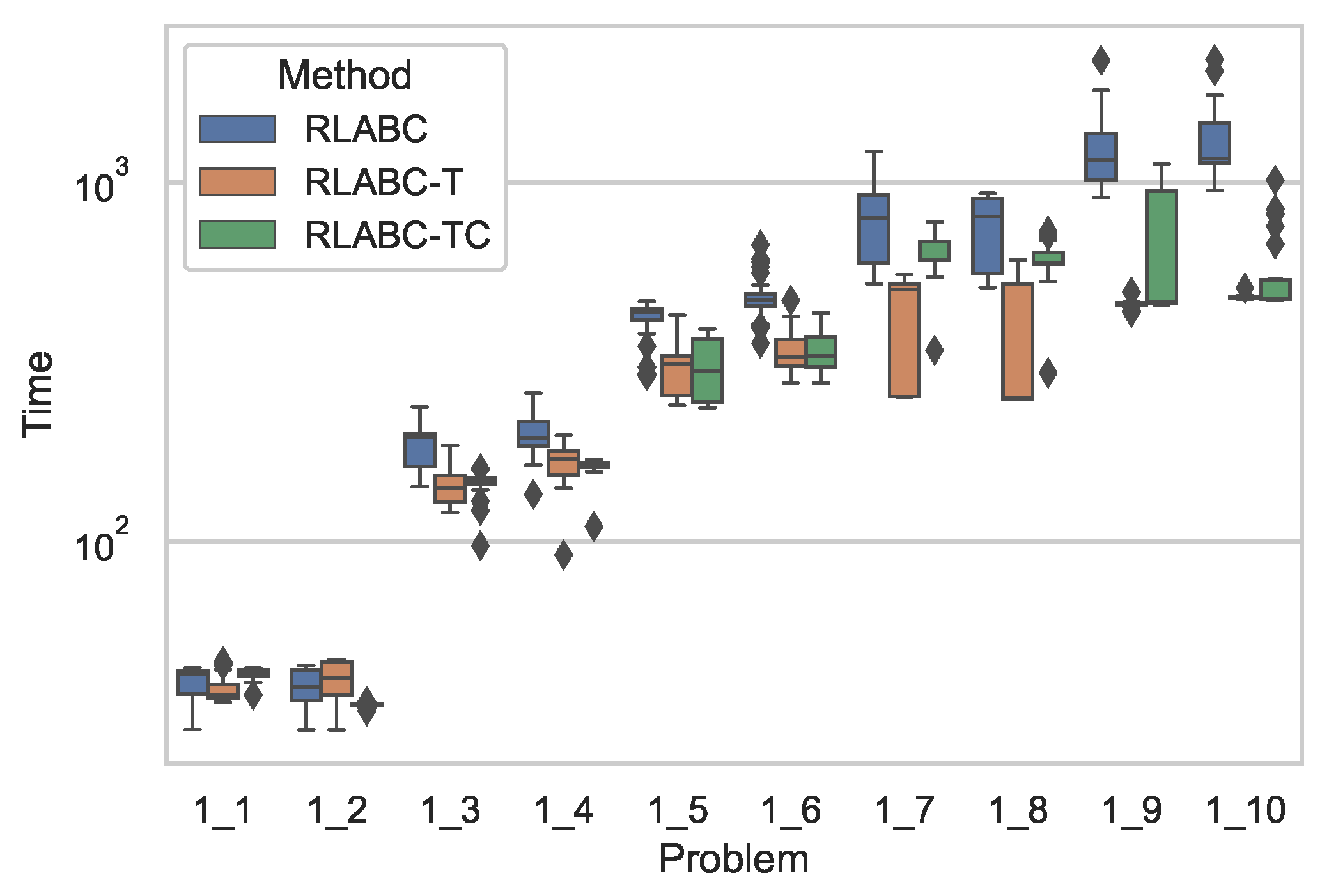
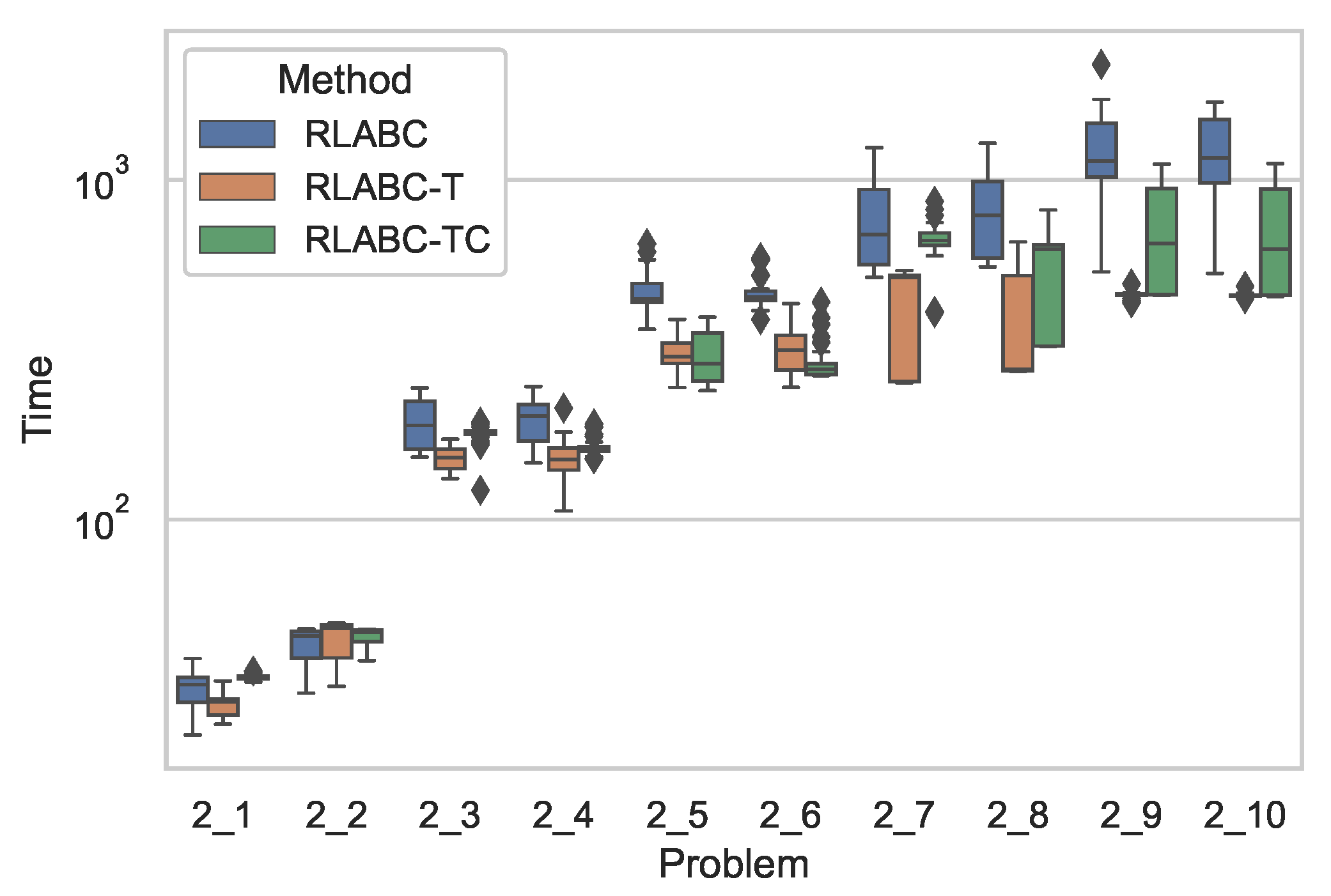
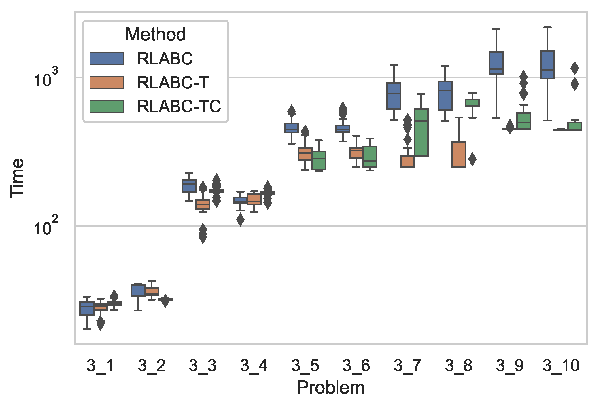
Figure 2 shows comparative results of the algorithms with respect to CPU time, while

Table 5. The results of statistical analysis on computational for Set₁ with respect to computational time.

	RLABC	RLABC-T		RLABC-TC
Instance No	Rank	Rank	Sign	Rank	Sign
1_1	2	3	+	1	−
1_2	2	1	+	3	−
1_3	3	2	+	1	+
1_4	3	1	+	2	+
1_5	3	1	+	2	+
1_6	3	1	+	2	+
1_7	3	2	+	1	+
1_8	3	2	+	1	+
1_9	3	2	+	1	+
1_10	3	2	+	1	+
Mean:	2.8	1.7		1.5

tabulates the statistical analysis of the results, where both the table and the figure demonstrate clear improvement by RLABC-T and RLABC-TC except for the cases of 1_1 and 1_2 instances, which are smaller in size. The growing size of the instances ascertains further that RLABC could not compete with the other variants. This suggests that when the problem dimension increases, RLABC has shown worse performance in terms of computational time. The results also indicate that RLABC-T and RLABC-TC remain competitive, but RLABC-TC has done slightly better than RLABC-T. Almost for all benchmarks except two instances, improvements on time performance are statistically meaningful. A similar situation applies to Figure 3 and Figure 4 and

Table 6. The results of statistical analysis for Set₂ with respect to computational time.

	RLABC	RLABC-T		RLABC-TC
	Rank	Rank	Sign	Rank	Sign
2_1	2	3	+	1	+
2_2	1	3	−	2	−
2_3	3	2	+	1	+
2_4	3	2	+	1	+
2_5	3	1	+	2	+
2_6	3	1	+	2	+
2_7	3	2	+	1	+
2_8	3	2	+	1	+
2_9	3	2	+	1	+
2_10	3	2	+	1	+
Mean:	2.7	2		1.3

and

Table 7. The results of statistical analysis for Set₃ with respect to computational time.

	RLABC	RLABC-T		RLABC-TC
	Rank	Rank	Sign	Rank	Sign
3_1	1	3	+	2	−
3_2	3	1	+	2	−
3_3	3	2	+	1	+
3_4	1	3	+	2	−
3_5	3	1	+	2	+
3_6	3	1	+	2	+
3_7	3	2	+	1	+
3_8	3	2	+	1	+
3_9	3	2	+	1	+
3_10	3	2	+	1	+
Mean:	2.6	1.9		1.5

, where the results by the algorithms applied to Set₂ and Set₃ are plotted and tabulated accordingly. These indicate that the comparisons with respect to the CPU time for all methods look similar to the cases of Set₁.

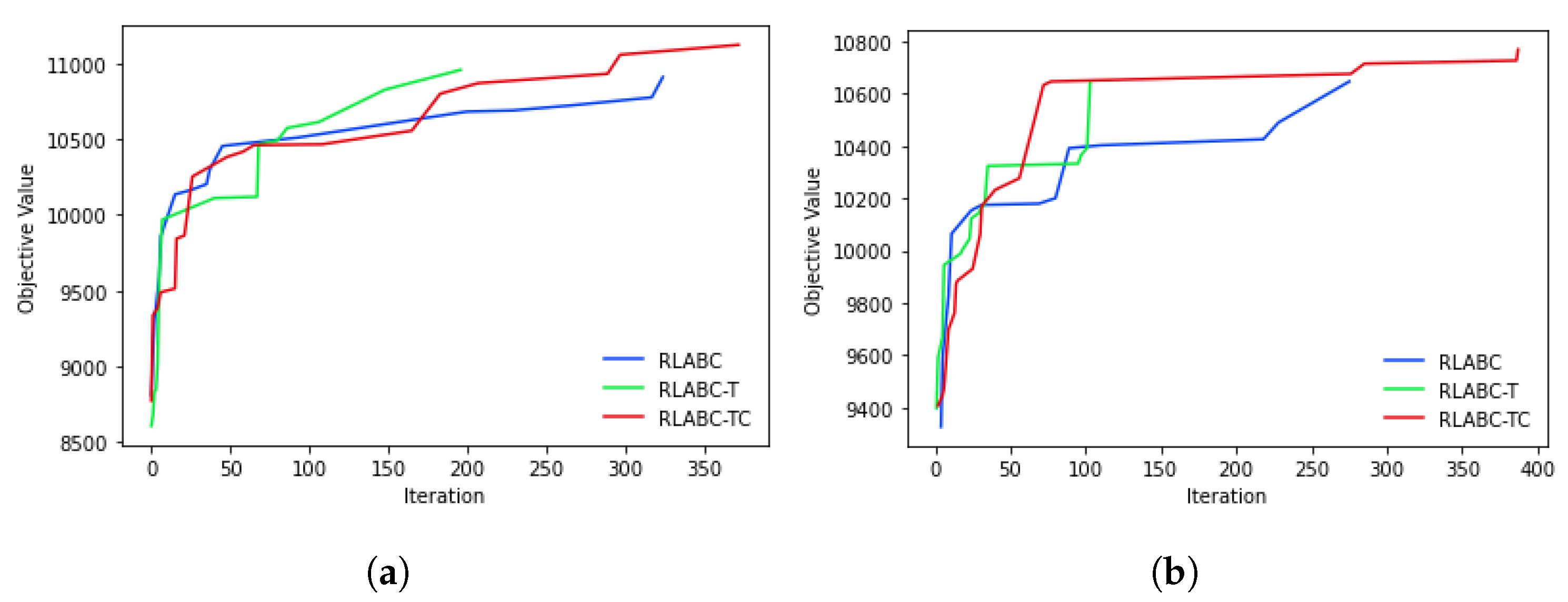
Figure 5 presents the convergence graphs of methods through the search process; Figure 5a shows the algorithms’ behaviour on a 400-dimensional problem, $2\_7$, and Figure 5b plots the performances on a 500-dimensional problem, $2\_9$. As can be seen in both figures, RLABC-T converges quicker than the other two but remains in local optima at around iteration 200. Meanwhile, RLABC-TC escapes that local optima in iterations such as 200, 300, and 350 in Figure 5a and in iterations around 80 and 250 in Figure 5b. On the other hand, RLABC gradually converges but stops after iteration 300 in both Figure 5a,b. This suggests that it is able to escape local optima at that points but cannot converge as RLABC-TC does. Both figures clarify that RLABC is outperformed by the other algorithms, while RLABC-TC converges better among all.

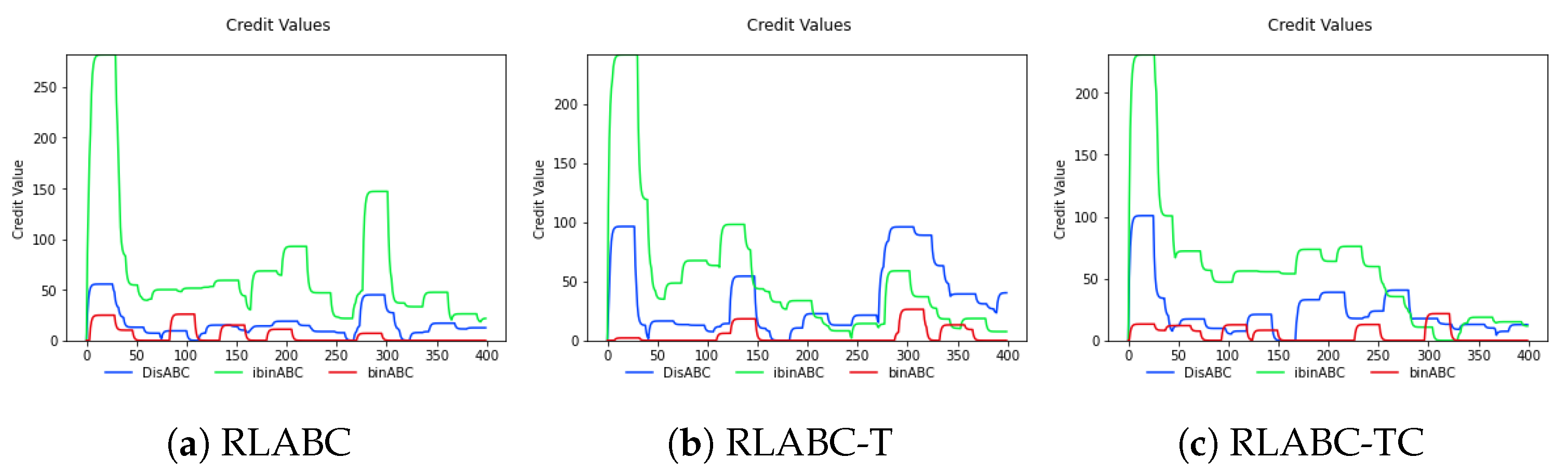
Figure 6 reflects the credit values gained by the three operators through iterations. As shown in the figure, all methods has slightly similar characteristics. ibinABC has obtained more credit from the start to the 200th iteration. The difference of methods is started from there. In the RLABC, ibinABC always has the most credited operator, while RLABC and RLABC have changed to DisABC and binABC.

In overall comparison, RLABC is a powerful algorithm that shows good performance than most of the state-of-art methods that are applied to the same problem, as in [4]. However, it does not allow transfer learning in problem solving. RLABC-T and RLABC-TC have improved the results not only in terms of solution quality but also the algorithm’s CPU time, demonstrating that the solution quality of the score is slightly better, while both RLABC-T and RLABC-TC significantly solve the problems much faster than RLABC. This experimentally approves the contribution of transfer learning in dynamically building an adaptive operator selection scheme. It is important to note that RLABC-T stops learning from new problem-solving runs, while RLABC-TC keeps updating the relevant centeroids of the corresponding clusters with upcoming new cases learned. The past experience jointly with undergoing learning remains beneficial in solving the problems faster without compromising the solution quality. The scope of this study has been kept to solve SUKP as an abstract combinatorial optimisation problem, which can be implemented into many real-world problems such as different variants of scheduling and timetabling problems. It is obvious that once a real-world problem can be solved with this approach as demonstrated, profit–loss analysis can be conducted to reveal the economical benefits.

The outperforming algorithm among three is RLABC-TC, which transfers previously gained experience into new runs and keeps learning active. It has been compared with some recently published very competitive state-of-art works—labelled as GA [28], BABC [32], binDE [33], and GPSO [31]—and the comparative results are plotted in Figure 7 on which all benchmark instances of the three sets have been considered, as shown on the horizontal axis of the graph, while the quality of the solution is indicated on the vertical axis. As a maximisation problem, the highest mean value is always delivered by RLABC-TC, which demonstrates the strength of the proposed approach.

5. Conclusions and Future Work

This article described how transfer learning was used in a reinforcement learning-based adaptive operator selection scheme incorporated in an ABC algorithm to tackle SUKP as a combinatorial optimisation problem. The ABC algorithm uses a pool of operators from which the adaptive operator selection scheme identifies the best-fitting operator for the current state of the problem and the search conditions. This helps search through the problem space in an efficient way. The operator selection scheme is developed and fine-tuned with the Q learning algorithm embedded and empowered with the “Hard-C-Means” clustering algorithm. The knowledge and experience gained through this process is transferred into the next runs to be utilised for faster approximation and better-quality solutions. The experimental results demonstrated that the transferred experience across runs helped achieve slightly better solution quality but significantly faster convergence. Both scenarios of keeping learning ON and OFF are tested, and it is observed that each has its own set of advantages and disadvantages. It is clearly observed that learning through a single run helps in solving problem instances in subsequent runs in a much shorter time. This is because the gained experience is used to select more complementary operators one after another, cutting the computational time, while the quality of the solution improves slightly or at least remains the same.

This study has considered the first level of experience and knowledge transfer in solving combinatorial optimisation problems, which implies training the agents in one run and utilising its gained experiences in the next runs. The next two levels, transfer across problem instances and problem types, remain as the future study, which is expected to achieve a significant breakthrough in building generic problem solvers. The proposed transfer learning method can be used to solve a wide range of real-world problems, which are applied to tackling in real-world applications, including but not limited to image recognition, speech recognition, and timetabling problems.

References

- Davis, L. Adapting operator probabilities in genetic algorithms. In Proceedings of the Third International Conference on Genetic Algorithms, San Francisco, CA, USA, 4–7 June 1989; pp. 61–69. [Google Scholar]
- Goldberg, D.E. Probability matching, the magnitude of reinforcement, and classifier system bidding. Mach. Learn. 1990, 5, 407–425. [Google Scholar] [CrossRef] [Green Version]
- Durgut, R.; Aydin, M.E. Adaptive binary artificial bee colony algorithm. Appl. Soft Comput. 2021, 101, 107054. [Google Scholar] [CrossRef]
- Durgut, R.; Aydin, M.E.; Atli, I. Adaptive operator selection with reinforcement learning. Inf. Sci. 2021, 581, 773–790. [Google Scholar] [CrossRef]
- Tan, C.; Sun, F.; Kong, T.; Zhang, W.; Yang, C.; Liu, C. A survey on deep transfer learning. In Proceedings of the International Conference on Artificial Neural Networks, Rhodes, Greece, 4–7 October 2018; Springer: Berlin/Heidelberg, Germany, 2018; pp. 270–279. [Google Scholar]
- Karaboga, D.; Akay, B. A comparative study of Artificial Bee Colony algorithm. Appl. Math. Comput. 2009, 214, 108–132. [Google Scholar] [CrossRef]
- Dorigo, M.; Birattari, M.; Stutzle, T. Ant colony optimization. IEEE Comput. Intell. Mag. 2006, 1, 28–39. [Google Scholar] [CrossRef]
- Kennedy, J.; Eberhart, R. Particle swarm optimization. In Proceedings of the ICNN’95-International Conference on Neural Networks, Perth, WA, Australia, 27 November–1 December 1995; Volume 4, pp. 1942–1948. [Google Scholar]
- Sutton, R.S.; Barto, A.G. Reinforcement Learning, Second Edition: An Introduction: An Introduction; The MIT Press: Cambridge, MA, USA, 2018. [Google Scholar]
- Sigaud, O.; Buffet, O. Markov Decision Processes in Artificial Intelligence; Wiley-IEEE Press: Hoboken, NJ, USA, 2010. [Google Scholar]
- Arulkumaran, K.; Deisenroth, M.P.; Brundage, M.; Bharath, A.A. Deep reinforcement learning: A brief survey. IEEE Signal Process. Mag. 2017, 34, 26–38. [Google Scholar] [CrossRef] [Green Version]
- Simon, D. Evolutionary Optimization Algorithms; John Wiley & Sons, Inc.: Hoboken, NJ, USA, 2013. [Google Scholar]
- Verheul, J. The Influence of Using Adaptive Operator Selection in a Multiobjective Evolutionary Algorithm Based on Decomposition. Master’s Thesis, Utrecht University, Utrecht, The Netherlands, 2020. [Google Scholar]
- Li, K.; Fialho, A.; Kwong, S.; Zhang, Q. Adaptive Operator Selection With Bandits for a Multiobjective Evolutionary Algorithm Based on Decomposition. IEEE Trans. Evol. Comput. 2014, 18, 114–130. [Google Scholar] [CrossRef]
- Torrey, L.; Shavlik, J. Transfer Learning. In Handbook of Research on Machine Learning Applications and Trends: Algorithms, Methods, and Techniques; Olivas, E.S., Guerrero, J.D.M., Martinez-Sober, M., Magdalena-Benedito, J.R., López, A.J.S., Eds.; IGI Global: Hershey, PA, USA, 2010; Chapter 11; pp. 242–264. [Google Scholar]
- Pan, S.J.; Yang, Q. A Survey on Transfer Learning. IEEE Trans. Knowl. Data Eng. 2010, 22, 1345–1359. [Google Scholar] [CrossRef]
- Lin, Q.; Liu, Z.; Yan, Q.; Du, Z.; Coello, C.A.C.; Liang, Z.; Wang, W.; Chen, J. Adaptive composite operator selection and parameter control for multiobjective evolutionary algorithm. Inf. Sci. 2016, 339, 332–352. [Google Scholar] [CrossRef]
- Zhang, Q.; Li, H. MOEA/D: A Multiobjective Evolutionary Algorithm Based on Decomposition. Trans. Evol. Comput. 2007, 11, 712–731. [Google Scholar] [CrossRef]
- Bischl, B.; Mersmann, O.; Trautmann, H.; Preuß, M. Algorithm selection based on exploratory landscape analysis and cost-sensitive learning. In Proceedings of the 14th Annual Conference on Genetic and Evolutionary Computation, Philadelphia, PA, USA, 7–11 July 2012; pp. 313–320. [Google Scholar]
- Hansen, N.; Auger, A.; Finck, S.; Ros, R. Real-Parameter Black-Box Optimization Benchmarking 2009: Experimental Setup; Research Report RR-6828; INRIA: Paris, France, 2009. [Google Scholar]
- Sallam, K.M.; Elsayed, S.M.; Sarker, R.A.; Essam, D.L. Landscape-based adaptive operator selection mechanism for differential evolution. Inf. Sci. 2017, 418, 383–404. [Google Scholar] [CrossRef]
- Handoko, S.D.; Nguyen, D.T.; Yuan, Z.; Lau, H.C. Reinforcement Learning for Adaptive Operator Selection in Memetic Search Applied to Quadratic Assignment Problem. In GECCO Comp’ 14, Proceedings of the Companion Publication of the 2014 Annual Conference on Genetic and Evolutionary Computation, Vancouver, BC, Canada, 12–16 July 2014; Association for Computing Machinery: New York, NY, USA, 2014; pp. 193–194. [Google Scholar]
- Chen, B.; Qu, R.; Bai, R.; Laesanklang, W. A variable neighborhood search algorithm with reinforcement learning for a real-life periodic vehicle routing problem with time windows and open routes. RAIRO-Oper. Res. 2020, 54, 1467–1494. [Google Scholar] [CrossRef]
- Aydin, M.E.; Öztemel, E. Dynamic job-shop scheduling using reinforcement learning agents. Robot. Auton. Syst. 2000, 33, 169–178. [Google Scholar] [CrossRef]
- Kiran, M.S.; Gündüz, M. XOR-based artificial bee colony algorithm for binary optimization. Turk. J. Electr. Eng. Comput. Sci. 2013, 21, 2307–2328. [Google Scholar] [CrossRef] [Green Version]
- Durgut, R. Improved binary artificial bee colony algorithm. Front. Inf. Technol. Electron. Eng. 2021, 22, 1080–1091. [Google Scholar] [CrossRef]
- Kashan, M.H.; Nahavandi, N.; Kashan, A.H. DisABC: A new artificial bee colony algorithm for binary optimization. Appl. Soft Comput. 2012, 12, 342–352. [Google Scholar] [CrossRef]
- Goldschmidt, O.; Nehme, D.; Yu, G. Note: On the set-union knapsack problem. Naval Res. Logist. (NRL) 1994, 41, 833–842. [Google Scholar] [CrossRef]
- Wu, C.; He, Y. Solving the set-union knapsack problem by a novel hybrid Jaya algorithm. Soft Comput. 2020, 24, 1883–1902. [Google Scholar] [CrossRef]
- He, Y.; Xie, H.; Wong, T.L.; Wang, X. A novel binary artificial bee colony algorithm for the set-union knapsack problem. Future Gener. Comput. Syst. 2018, 78, 77–86. [Google Scholar] [CrossRef]
- Ozsoydan, F.B.; Baykasoglu, A. A swarm intelligence-based algorithm for the set-union knapsack problem. Future Gener. Comput. Syst. 2019, 93, 560–569. [Google Scholar] [CrossRef]
- Ozturk, C.; Hancer, E.; Karaboga, D. A novel binary artificial bee colony algorithm based on genetic operators. Inf. Sci. 2015, 297, 154–170. [Google Scholar] [CrossRef]
- Engelbrecht, A.P.; Pampara, G. Binary differential evolution strategies. In Proceedings of the 2007 IEEE Congress on Evolutionary Computation, Singapore, 25–28 September 2007; pp. 1942–1947. [Google Scholar]
Figure 1.
Reinforcement learning-based adaptive operator selection scheme embedded in ABC algorithm. Input X is presented to the ’Operator Selection’ unit and merged with the output O generated before and passed to ’Cluster Update’ unit to make operator a selected. Once done, operator a generates a new O and evaluates the quality of solution with . Meanwhile, X and O are passed to the ’Reward Generation’ unit to produce r and forwarded to ’Cluster Update’ to adapt with the new knowledge. This repeats throughout the complete search process.
Figure 2.
Comparative results with respect to computational time by all three (RLABC, RLABC-T, RLABC-TC) algorithms for Set1 benchmarks.
Figure 3.
Comparative results with respect to computational time by all three (RLABC, RLABC-T, RLABC-TC) algorithms for Set2 benchmarks.
Figure 4.
Comparative results with respect to computational time by all three (RLABC, RLABC-T, RLABC-TC) algorithms for Set3 benchmarks.
Figure 5.
Convergence level attained by each operator while solving (a) 2_7 problem instance and (b) 2_9 problem instance.
Figure 6.
The change of credit levels gained by each operator while solving some benchmark instances through iterations; (a) credits gained with the RLABC algorithm, (b) credits gained with the RLABC-T algorithm, and (c) credits gained with the RLABC-TC algorithm.
Figure 7.
Comparative results by the proposed approach, RLABC-TC, and the state-of-art methods, GA [28], BABC [32], binDE [33], and GPSO [31], on benchmark instances in Set1, Set2, and Set3.