

Investigating Errors Observed during UAV-Based Vertical Measurements Using Computational Fluid Dynamics

1
Department of Chemical Engineering, University of Utah, Salt Lake City, UT 84112-9203, USA
2
Department of Physics and Astronomy, Weber State University, Ogden, UT 84408-2508, USA
*
Author to whom correspondence should be addressed.
Drones 2022, 6(9), 253; https://doi.org/10.3390/drones6090253
Submission received: 8 August 2022
/
Revised: 5 September 2022
/
Accepted: 6 September 2022
/
Published: 13 September 2022
(This article belongs to the Special Issue Unmanned Aerial Vehicles in Atmospheric Research)
Abstract
:Unmanned Aerial Vehicles (UAVs) are a popular platform for air quality measurements. For vertical measurements, rotary-wing UAVs are particularly well-suited. However, an important concern with rotary-wing UAVs is how the rotor-downwash affects measurement accuracy. Measurements from a recent field campaign showed notable discrepancies between data from ascent and descent, which suggested the UAV downwash may be the cause. To investigate and explain these observed discrepancies, we use high-fidelity computational fluid dynamics (CFD) simulations to simulate a UAV during vertical flight. We use a tracer to model a gaseous pollutant and evaluate the impact of the rotor-downwash on the concentration around the UAV. Our results indicate that, when measuring in a gradient, UAV-based measurements were ∼50% greater than the expected concentration during descent, but they were accurate during ascent, regardless of the location of the sensor. These results provide an explanation for errors encountered during vertical measurements and provide insight for accurate data collection methods in future studies.
1. Introduction
Unmanned Aerial Vehicles (UAVs), also called drones, are a useful tool in air quality monitoring given their ability to obtain data with high spatial and temporal resolution. Rotary-wing UAVs are a popular platform for vertical measurements given their ability to fly in any direction and hover. Multiple studies have used rotary-wing UAVs for vertical measurements to study various species and pollutants in the atmosphere [1,2,3,4,5], to study traffic emissions [6,7], and to estimate the height of the planetary boundary layer [8,9]. An important concern when using rotary-wing UAVs is how the downwash from the propellers affects measurement accuracy.
Previous studies have investigated the strength of the airflow around the UAV using wind tunnel and plume experiments to visualize the airflow with smoke or particles and measure the air speed around the rotors [3,10,11,12,13]. Some studies have also used computational fluid dynamics (CFD) simulations as a means of estimating where the airflow and effects of the rotors are the strongest [10,14,15,16]. In [10], the airflow around a UAV with six propellers was simulated using CFD and they found that the region of air influenced by the UAV propellers is roughly cylindrical, with a radius of two meters that extends two meters above and eight meters below the UAV. CFD was also used by [14] to study a six-propeller UAV and it was found that the residence time of air in the sampling region under the center of the UAV was small, indicating that measurements from that region were representative of the surrounding air. Other studies evaluating the airflow around a UAV have concluded that placing a sensor above the center of the UAV or outside the rotors is best to avoid disturbance from the propellers [13,15].
Simulations of UAVs for agricultural applications have shown that the airflow changes significantly depending on the flight direction and speed [17,18]. This suggests that flight direction and speed should be taken into account when considering UAV-based air quality measurements. However, all of the aforementioned studies focused on air quality have only evaluated the airflow around a UAV under hover conditions. Similarly, most experimental studies that have compared a UAV-based instrument to another reference monitor do so while hovering [5,19]. One study did compare UAV-based vertical measurements of ozone to measurements from a tethered balloon and found reasonable agreement between the two platforms [1]. However, the measurements were performed during a relatively uniform period in the ozone distribution. Thus, previous conclusions and recommendations may not be sufficient to ensure accuracy of UAV-based measurements in every case. For example, vertical measurements of black carbon presented by [20] showed notable discrepancies between data from ascent versus descent even though guidelines for sensor placement from previous studies were followed.
Similar to [20], we have observed inconsistencies in vertical ozone profiles collected using a UAV. These experimental observations prompted us to investigate the effect of the downwash and airflow further. Our goal in this study is to use high-fidelity CFD simulations to investigate and explain how the downwash can affect vertical measurements by simulating a UAV during vertical flight [21]. Our hypothesis is that there will be more turbulent mixing and possibly recirculation during descent than during ascent which could interfere with measurements. Our simulations differ from previous work in that we use a large-eddy simulation (LES) methodology which resolves more of the turbulence and mixing caused by the rotors compared to the Reynolds-averaged Navier–Stokes (RANS) formulation used by other studies [14,15,16]. We also perform a transient rather than steady-state analysis to evaluate the UAV while it is flying and sampling a gaseous pollutant. To the best of our knowledge, this work is the first to simulate a UAV during vertical flight conditions. This work will provide insight into past observations as well as prevent future discrepancies and errors in field measurements.
Details regarding the experiments that prompted this study are provided in the methods section as well as an overview of the governing equations and models used in the CFD simulations. Then, the results of our simulations are presented, highlighting the differences in airflow and scalar mixing between ascent and descent. Finally, the discrepancies observed in our prior experiments are explained in light of the simulation results and recommendations are given to avoid similar discrepancies in future measurements and provide insight for sensor placement.
2. Materials and Methods
The data that prompted this investigation were part of a field campaign to study the evolution and transport of summertime ozone in northern Utah, USA. Discrepancies were observed between data from ascent and descent from flights during the morning hours when there is a gradient in the vertical ozone profile. The data were collected using a rotary-wing drone with an ozonesonde attached beneath it. The model 2ZV7-ECC ozonesonde was prepared for flights over a period of several days according to the operations manual [22]. During this period, the electrolytes were refreshed and the instrument was run while alternating between clean air (no ozone) and air at an ozone concentration of 50% of full scale for ten to twenty minutes. Over time, these activities lower the background current of the cell. During the last cycle, the background current is measured along with the pump performance and the cell’s response to a step change in input gases. These values are then used to process the raw data gathered during flights.
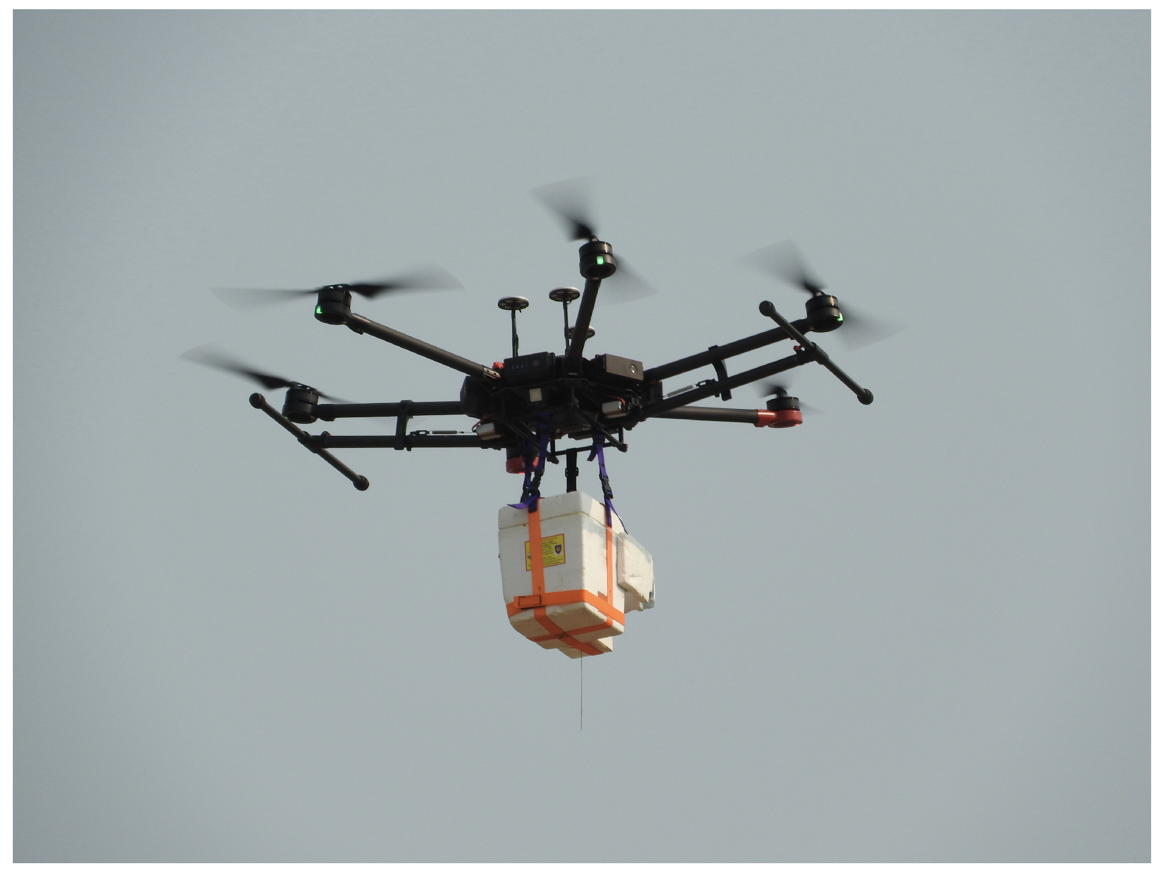
The UAV used in this study was a DJI Matrice 600 Pro (M600) which has been commonly used in other studies for similar measurements of vertical ozone distributions [2,8,23]. This UAV has six propellers that are each about 53 cm in diameter and can carry a payload of up to 6.5 kg. Custom straps were used to secure the payload below the UAV (Figure 1). Ozone mixing ratio was measured using an ozonesonde and transmitted to a ground station via radiosonde. Data were recorded at one-second intervals. During each flight, the UAV ascended and descended at a constant speed of approximately 1 m/s.
Computational Fluid Dynamics Simulations
Our simulations attempt to mimic the experimental setup and procedure as closely as possible. An in-house CFD code, Wasatch, was used to perform simulations of the UAV during vertical flight. Wasatch is a finite volume, large-eddy simulation (LES) software that solves the incompressible and low-Mach Navier–Stokes equations on a structured, uniform grid ([21]). Wasatch is a highly efficient and flexible parallel CFD code that has been used to study very complex turbulent flows including multiphase flows with precipitation [24], turbulence decay [25], and respiratory aerosol transport in orchestras [26], making it very suitable for this study. We consider the LES-filtered, incompressible, constant-density Navier–Stokes equations
where is the filtered velocity, is the density, is the filtered pressure, is the filtered stress tensor, and is the subgrid stress tensor. Subgrid stresses were modeled using the dynamic Smagorinsky model ([27,28]).
To model the UAV propellers, a momentum source term that represents the thrust per unit volume for each rotor is added to Equation (2) in the location of the rotors (see Figure 2). This approach is similar to actuator disk models commonly used for helicopters and wind turbines [29,30]. Thrust is caused by the pitch of the rotor blades. As each neighboring rotor counter-rotates, the net rotational motion to the air column goes to zero and was not accounted for in our simulations. However, we do account for the angle of the UAV arms by distributing the total force in the axial direction (downward) and radial direction (away from the UAV). The thrust force necessary for the UAV to hover in the air was calculated based on the combined weight of the UAV and its payload. Assuming the combined weight of the UAV and payload is balanced only by the thrust from the rotors, then
where is the gravitational force (Newtons) on the drone, is the mass (kg) of the drone, m/s is the acceleration due to gravity, N is the number of rotors, and is the thrust force produced by one rotor. Subsequently, the thrust per unit volume for each rotor is
where is the volume swept by a rotor with R and designating the rotor radius and thickness, respectively. The main frame of the UAV and the payload were modeled using simplified geometries but the UAV landing gear was not included (Figure 2).
Transport of a gaseous pollutant (i.e., ozone) was modeled using an advection–diffusion transport equation
where is the pollutant concentration, and are the molecular and turbulent diffusivities of , respectively, and is the fluid viscosity. The turbulent Schmidt number is taken to be [31,32]. We simulated a vertical flight through an air column with a linear gradient in pollutant concentration. To model the concentration measured by the ozonesonde, we used the concentration value from the simulation under the center of the UAV and at two other potential locations for the instrument intake: above the UAV and outside of the rotors. Ozone is a reactive pollutant and is generally formed in the morning hours through a series of photochemical reactions. We did not account for reactivity or formation in our simulations because the duration of the experimental flights (5 min) was much shorter than the timescale for ozone formation (∼10 ppb per h) [33]. However, when performing longer flights, reactivity and formation should be considered in the model.
The domain in our simulation was 6× 6 × 5 m (length × width × height) and the grid resolution was 2.5 cm in the x- and y- directions and 1.25 cm in the z-direction with a total of 23 million grid cells. The scalar variable was initialized to 0 for ascent or 1 for descent and a time-dependent Dirichlet boundary condition was applied on the scalar variable at the top (ascent) or bottom (descent) boundary to create a linear gradient of . For ascent, an inflow velocity of 1 m/s was set at the top boundary and an outflow condition was used at the bottom of the domain. For descent, the inflow was at the bottom of the domain and the outflow at the top. The side walls of the domain were set to mimic a calm atmosphere with a gentle inflow of 0.5 m/s. Calculations were run to a simulation time of 30 s.
3. Results
As stated previously, the purpose of this work was to use CFD to simulate vertical flight for a rotary-wing UAV and provide insight into the inconsistencies observed in our experimental data. Sample profiles from our experiments are shown in Figure 3. The profiles all show higher mixing ratios during descent compared to ascent. The differences between the ascent and descent profiles decrease as the profiles becomes more uniform later in the morning.
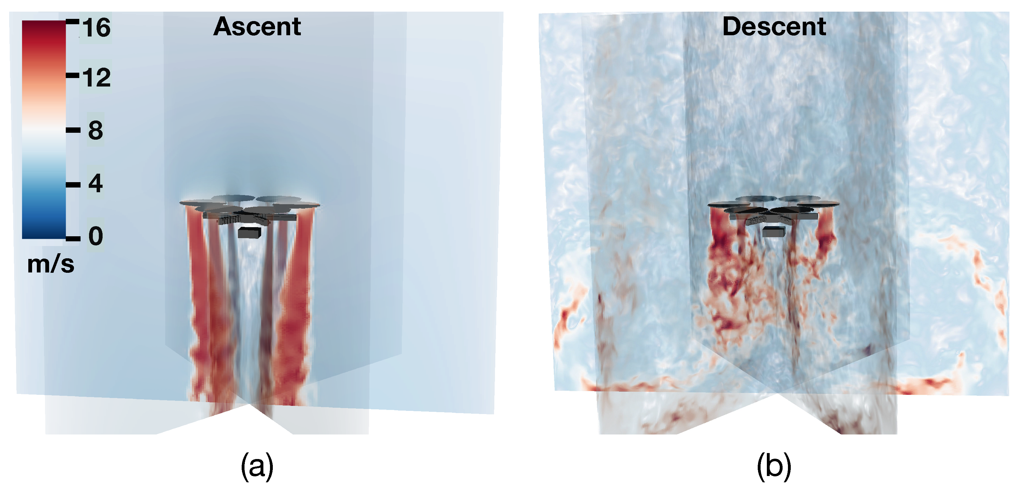
To investigate the discrepancies observed in our experimental data, we evaluated the airflow and pollutant concentration around the drone for two cases: ascent and descent. The airflow between the two cases differs greatly as shown in Figure 4. During ascent, there is strong airflow underneath the UAV rotors with air speeds of approximately 15 m/s (Figure 4a). The air flow around the payload is weaker with speeds up to 5 m/s, and the airflow outside the UAV rotors is relatively undisturbed. During descent, the airflow is also fastest under the drone rotors, however, the airflow around the drone is more transient and chaotic than during ascent. These disturbances are a result of the drone passing through its own wake as it descends.
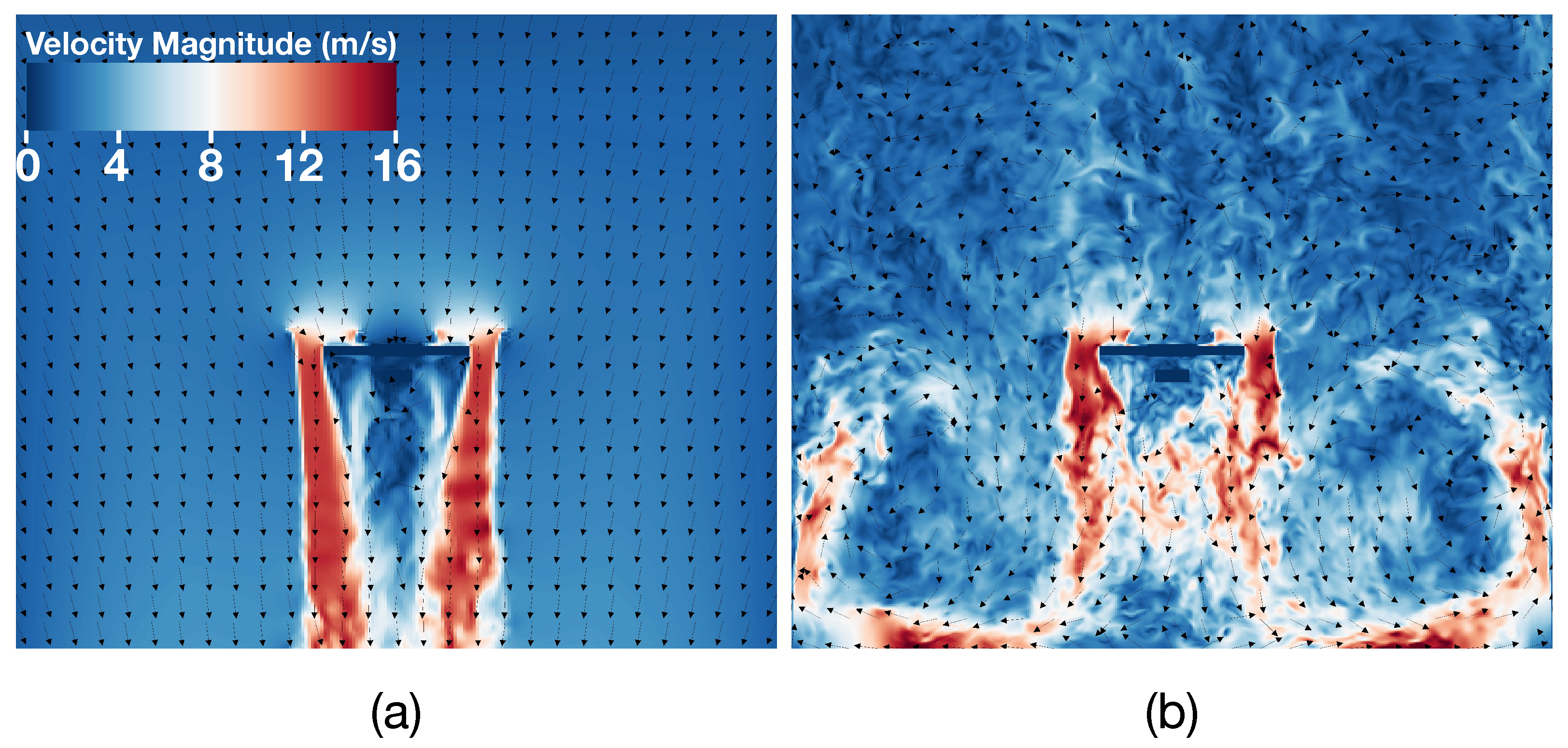
In addition to the increased air disturbance, Figure 5b shows how some of the air from the wake of the drone can recirculate through the rotors during descent. This suggests that during descent, the payload may be sampling from the same volume of air multiple times rather than fresh, new air from above the drone or outside of the wake. During ascent, this recirculation is non-existent because the drone is flying upwards away from its own wake. The velocity vectors in Figure 5a show that new air is constantly flowing from above the drone into the region around the payload. The residence time in the region around the payload is in the order of 1–5 s which is in agreement with values reported in the literature [14] and is the same as the sampling timescale of the ozonesonde (∼1 s) from which the experimental data were collected. This indicates that the data from the ozonesonde during ascent should accurately represent spatial variations in ozone concentration.
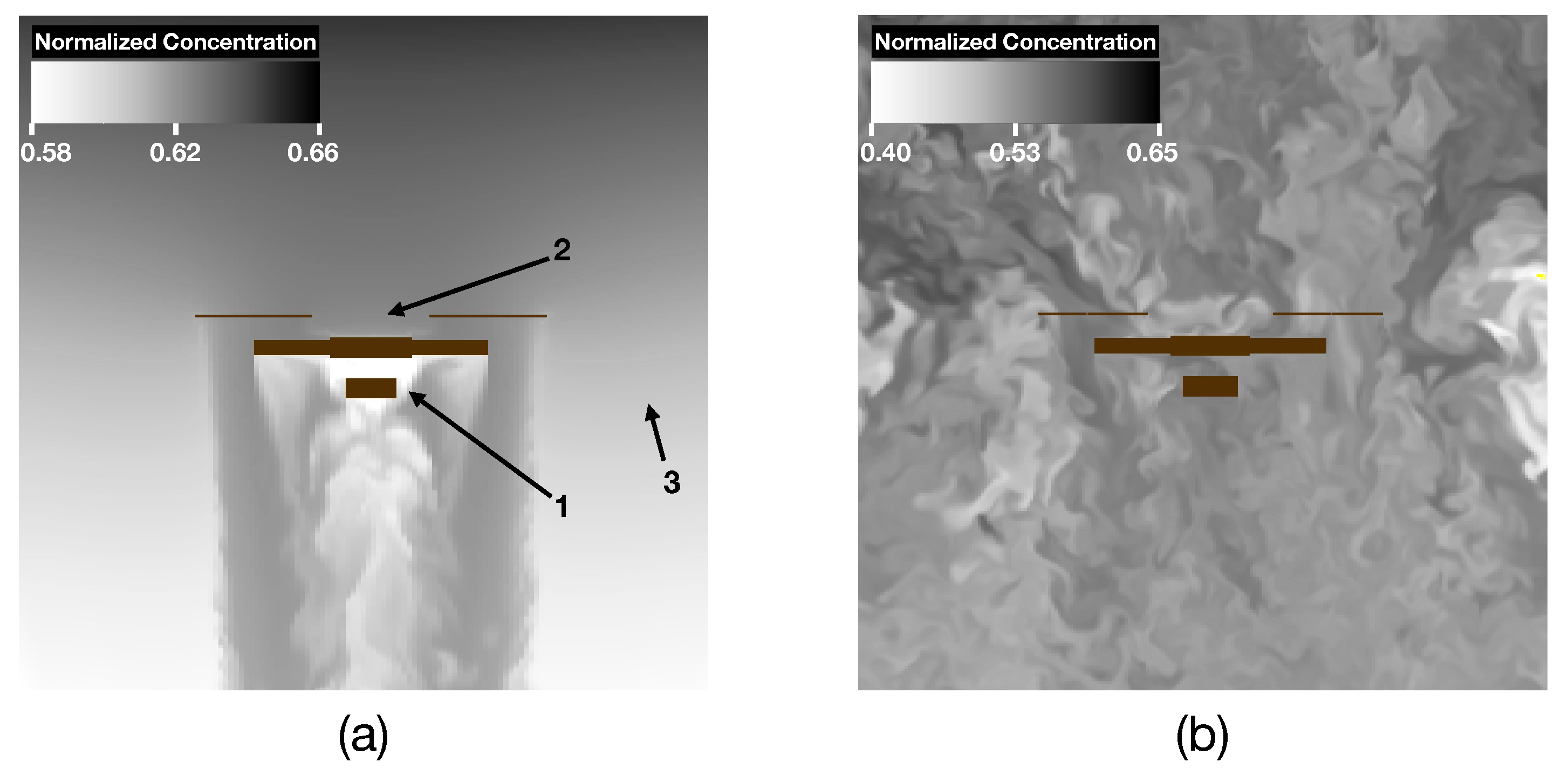
To evaluate the effects of the drone rotors on gaseous pollutant measurements, we tracked a tracer (passive scalar) in our simulations. The patterns observed in the normalized scalar concentration are similar to those seen in the airflow. During ascent, the instantaneous normalized scalar concentration under the rotors is slightly higher than the concentration outside of the rotors (approximately 0.633 and 0.617, respectively) due to the fact that the rotors draw fresh air from above the drone (Figure 6a). The normalized concentration around the payload is comparable to the other regions (∼0.627). A linear gradient in the concentration is observed in the region outside of the rotors. During descent, there is notable mixing and some gradients in the concentration but the linear profile that is expected has been disturbed by the rotors (Figure 6b).
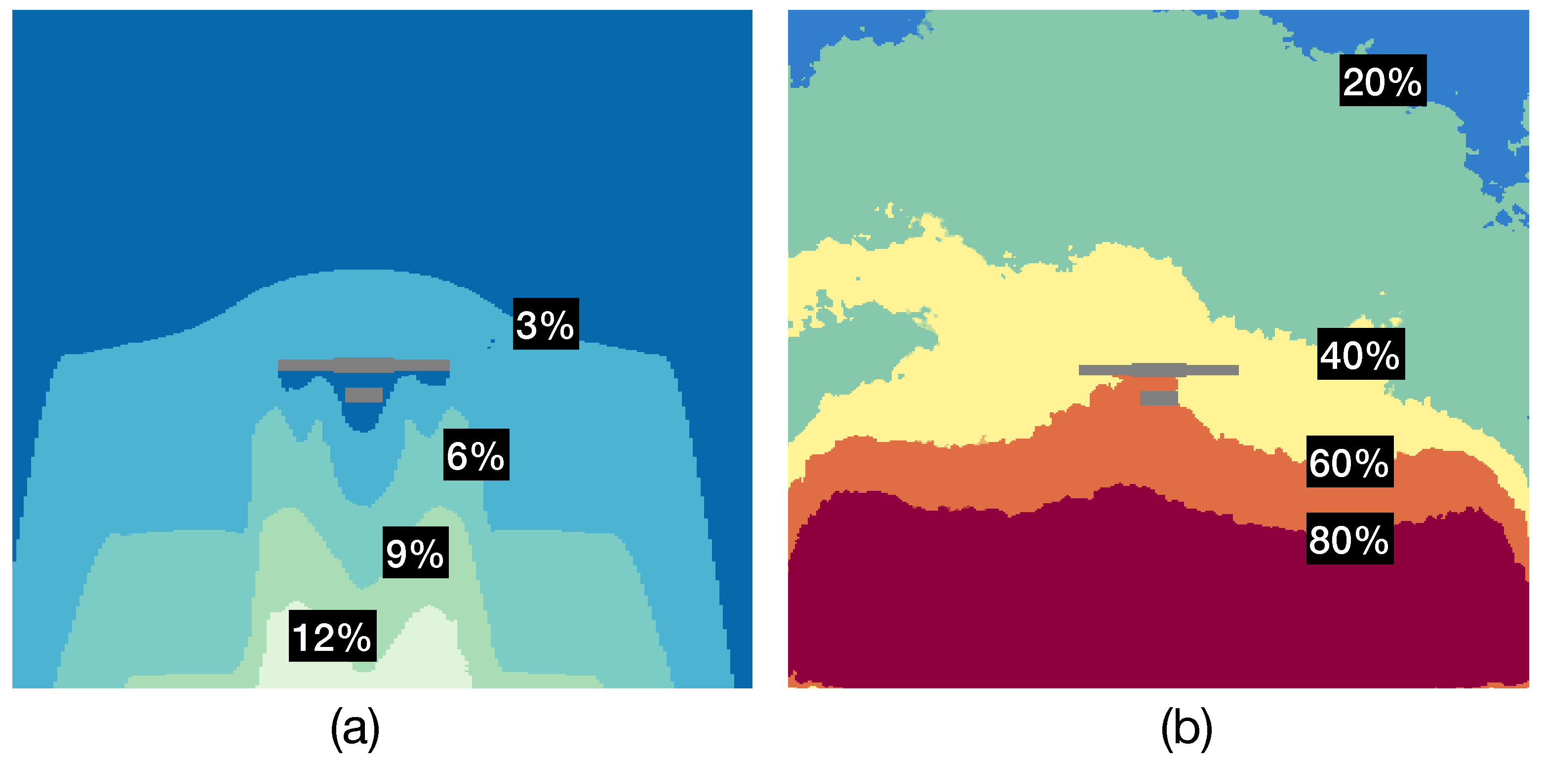
By comparing the scalar concentration around the drone to the expected concentration based on the imposed boundary conditions, we calculated the relative error caused by the rotors as
where is the expected concentration and is the actual concentration. The error was averaged over the last 10 s of the simulation and a slice was taken through the middle of the domain (Figure 7). Discrete regions are shown with the concentrations at the borders between regions labeled. For both ascent and descent, the maximum relative error is under the drone in the wake. However, the maximum relative error during ascent is only 12% whereas during descent the maximum relative error reaches values greater than 100%. Around the UAV, the relative error is small during ascent, ranging from 3–6% (Figure 7a), but during descent, the relative error around the UAV ranges from 40–60% (Figure 7b). This suggests that measurements during descent will be highly compromised by the disturbance caused by the rotors while measurements from ascent will be largely unaffected.
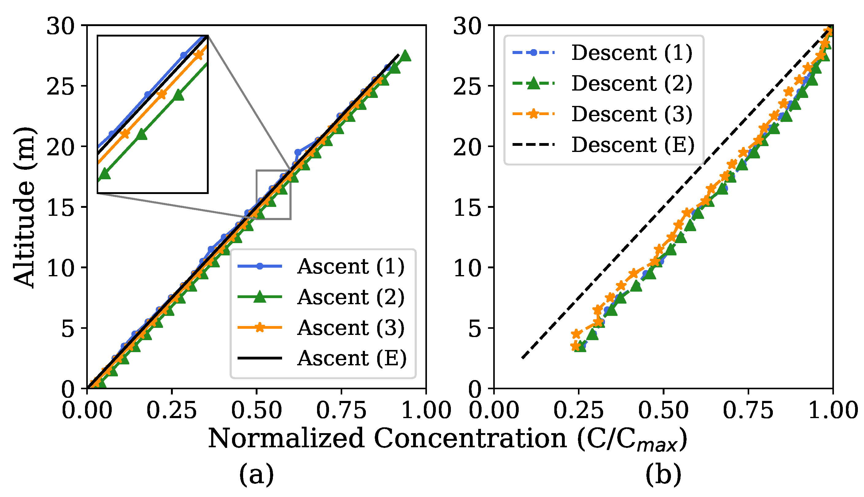
In order to investigate the influence of sensor or intake location, three potential intake tube locations were chosen in the simulation: (1) next to the payload, (2) above the drone, (3) outside the rotors. These locations are marked in Figure 6a. These locations were chosen based on the normal location of the intake tube and recommendations from other studies [13,15,16]. Figure 8 shows the normalized concentration plotted against altitude for each or the locations chosen along with the expected profile based on the imposed boundary conditions. The curves during ascent are all clustered together around the expected profile with negligible differences between each location, indicating both good accuracy and precision (see Figure 8a). However, while the curves for descent are also clustered together with small differences between locations, all three locations are shifted to the right of the expected profile, indicating good precision but poor accuracy (see Figure 8b). This indicates that the concentrations measured during descent will be higher than expected regardless of sensor placement. The shift in the descent curves is similar to the trend observed in our experimental data.
4. Discussion
Our results show that measurements of gaseous pollutants using a UAV may be inaccurate during descent due to the mixing and recirculation caused by the rotors. The trends in our simulations between ascent and descent are similar to those observed in our experiments, which suggests that mixing from the rotors was responsible for the discrepancies in our experimental data. To reduce error in vertical measurements, our results suggest that data should be collected during ascent only. This differs from some previous studies that have used data collected during descent after eliminating outliers [16,23]. Using data from descent may not have been problematic in those studies given that many of the profiles they measured were relatively uniform. As our results showed, measurements during descent are most affected when measuring along a gradient in concentration.
Our results also indicate that below the UAV is a suitable location for the instrument or intake tube. For vertical measurements, we saw no differences in our simulation data at the location above the UAV or outside of the rotors when compared to below the drone. Our results suggest that for the UAV used in this study, the rotors are far enough from the UAV center such that the airflow under the UAV center is mild compared to the airflow directly under the rotors. Based on these results, we recommend placing a sensor or sensor intake below the UAV center as this is the normal location for a payload and is least likely to cause instability during flight. However, it may be advantageous or necessary in certain cases to extend the intake to one of the other locations suggested by previous studies depending on the size of the UAV, the size and shape of the payload, or the instrument sensitivity [13,15].
Some of the limitations of our study include the low-cost model used for the UAV rotors and possible boundary effects due to the size of our domain. The model used to represent the rotors creates a constant thrust force to balance the weight of the UAV and payload which creates a velocity in the vertical direction. The model does not account for rotation in the flow or vortices shed by the wings or at the wing tips. These effects are especially relevant when designing a UAV and measuring the pressure distribution or thrust force generated by the rotor. In our study, we are mainly concerned with the bulk airflow around the UAV and its impact on air quality measurements. Since vortices shed from the rotors will have a secondary effect on the bulk airflow, it is reasonable to neglect these effects in our simulations. In addition, our simulations show that the airflow around the payload is weak compared to the flow directly under the rotors, and we were able to confirm this experimentally using an anemometer. We also used a tell-tale ribbon attached to a thin pole to indicate the direction of airflow under the UAV and observed good agreement with our simulations with strong downward flow under the rotors and flow upwards under the UAV around the payload. The airflow around the payload might be stronger when using a smaller drone with rotors that are closer together. In that case, it may be necessary to use a more accurate model.
Setting boundary conditions that accurately model atmospheric conditions can be challenging and expensive. One approach is impose turbulent inflow data from a precursor simulation at the boundaries. Another possibility is to use a large domain such that the boundaries are far from the region of interest. To obtain results in a reasonable amount of time, we applied simpler Dirichlet boundary conditions with flow moving either downwards or upwards to mimic ascent and descent, respectively. The boundaries in our domain were over two meters away from the UAV; however, they may still have an effect on the airflow within the domain. For example, during descent, the vertical flow at the boundary may cause the stronger recirculation in the wake than would normally occur. Given the good agreement between the trends observed in our simulations and the experimental observations (see Figure 3), these effects are likely minor and do not compromise the results of our study.
5. Conclusions
In summary, this work provides an explanation of errors observed during vertical measurements using a rotary-wing UAV and guidelines to avoid similar errors in vertical measurements. We use CFD simulations to model a UAV during a vertical flight while measuring a gaseous pollutant. We found that the rotors cause vertical mixing which can smooth gradients in the atmosphere and introduce bias into measurements made during descent. We also found that errors occurred during descent regardless of whether the instrument intake tube is placed below the UAV, above the UAV, or extended to the side. The effects of the rotors are not observed during ascent, nor if the concentration is uniform vertically.
Based on our findings, we recommend that data should only be collected during ascent for vertical measurements. Disregarding measurements during descent and descending quickly can help save time and battery life and allow for more efficient measurements. We also recommend placing the payload and intake tube below the center of the UAV to avoid any issues with UAV stability; however, placement of the payload may vary based on size, shape and other payload-specific requirements.
This study demonstrates how CFD can be a powerful tool to inform air quality and other mobile measurements using UAVs. Unlike previous studies, our simulations capture the instantaneous effects of turbulent mixing caused by the rotors, as well as model gaseous pollutant transport during ascent and descent. Future work could include modelling different flight and measurement scenarios such as forward flight or hover while measuring in a plume or from a localized source.
Author Contributions
Conceptualization, H.H., J.S. and T.S.; methodology, H.H., J.P., J.S. and T.S.; software, H.H. and T.S.; validation, H.H. and T.S.; formal analysis, H.H.; investigation, H.H., J.P., J.S. and T.S.; resources, J.P., J.S., T.S.; data curation, H.H., J.P., J.S. and T.S.; writing—original draft preparation, H.H.; writing—review and editing, H.H., J.P., J.S. and T.S.; visualization, H.H. and T.S.; supervision, J.P., J.S. and T.S.; project administration, J.S. and T.S.; funding acquisition, J.S. and T.S. All authors have read and agreed to the published version of the manuscript.
Funding
Funding for this work was provided by the National Science Foundation through an EAGER award (Grant No. EAGER 2125997), by the Utah Department of Environmental Quality through the Division of Air Quality, and the Department of Chemical Engineering at the University of Utah.
Institutional Review Board Statement
Not applicable.
Informed Consent Statement
Not applicable.
Data Availability Statement
Data from this study is available from the corresponding author upon request.
Acknowledgments
The authors acknowledge support from the Center for High Performance Computing at the University of Utah for providing the computational resources used in this work.
Conflicts of Interest
The authors declare no conflict of interest.
References
- Chen, Q.; Wang, D.; Li, X.; Li, B.; Song, R.; He, H.; Peng, Z. Vertical Characteristics of Winter Ozone Distribution within the Boundary Layer in Shanghai Based on Hexacopter Unmanned Aerial Vehicle Platform. Sustainability 2019, 11, 7026. [Google Scholar] [CrossRef]
- Chen, Q.; Li, X.B.; Song, R.; Wang, H.W.; Li, B.; He, H.D.; Peng, Z.R. Development and utilization of hexacopter unmanned aerial vehicle platform to characterize vertical distribution of boundary layer ozone in wintertime. Atmos. Pollut. Res. 2020, 11, 1073–1083. [Google Scholar] [CrossRef]
- Crazzolara, C.; Ebner, M.; Platis, A.; Miranda, T.; Bange, J.; Junginger, A. A new multicopter-based unmanned aerial system for pollen and spores collection in the atmospheric boundary layer. Atmos. Meas. Tech. 2019, 12, 1581–1598. [Google Scholar] [CrossRef]
- Schuyler, T.J.; Bailey, S.C.C.; Guzman, M.I. Monitoring Tropospheric Gases with Small Unmanned Aerial Systems (sUAS) during the Second CLOUDMAP Flight Campaign. Atmosphere 2019, 10, 434. [Google Scholar] [CrossRef]
- Wang, T.; Han, W.; Zhang, M.; Yao, X.; Zhang, L.; Peng, X.; Li, C.; Dan, X. Unmanned Aerial Vehicle-Borne Sensor System for Atmosphere-Particulate-Matter Measurements: Design and Experiments. Sensors 2020, 20, 57. [Google Scholar] [CrossRef]
- Weber, K.; Heweling, G.; Fischer, C.; Lange, M. The Use of an Octocopter UAV for the Determination of Air Pollutants—A Case Study of the Traffic Induced Pollution Plume Around a River Bridge in Duesseldorf, Germany. Int. J. Educ. Learn. Syst. 2017, 2. [Google Scholar]
- Zheng, T.; Li, B.; Li, X.B.; Wang, Z.; Li, S.Y.; Peng, Z.R. Vertical and horizontal distributions of traffic-related pollutants beside an urban arterial road based on unmanned aerial vehicle observations. Build. Environ. 2021, 187, 107401. [Google Scholar] [CrossRef]
- Guimarães, P.; Ye, J.; Batista, C.; Barbosa, R.; Ribeiro, I.; Medeiros, A.; Souza, R.; Martin, S.T. Vertical Profiles of Ozone Concentration Collected by an Unmanned Aerial Vehicle and the Mixing of the Nighttime Boundary Layer over an Amazonian Urban Area. Atmosphere 2019, 10, 599. [Google Scholar] [CrossRef]
- Guimarães, P.; Ye, J.; Batista, C.; Barbosa, R.; Ribeiro, I.; Medeiros, A.; Zhao, T.; Hwang, W.C.; Hung, H.M.; Souza, R.; et al. Vertical Profiles of Atmospheric Species Concentrations and Nighttime Boundary Layer Structure in the Dry Season over an Urban Environment in Central Amazon Collected by an Unmanned Aerial Vehicle. Atmosphere 2020, 11, 1371. [Google Scholar] [CrossRef]
- Haas, P.Y.; Balistreri, C.; Pontelandolfo, P.; Triscone, G.; Pekoz, H.; Pignatiello, A. Development of an unmanned aerial vehicle UAV for air quality measurement in urban areas. In Proceedings of the 32nd AIAA Applied Aerodynamics Conference, AIAA AVIATION Forum, Atlanta, GA, USA, 16–20 June 2014. [Google Scholar] [CrossRef]
- Hedworth, H.A.; Sayahi, T.; Kelly, K.E.; Saad, T. The effectiveness of drones in measuring particulate matter. J. Aerosol Sci. 2021, 152, 105702. [Google Scholar] [CrossRef]
- Black, O.; Chen, J.; Scircle, A.; Zhou, Y.; Cizdziel, J.V. Adaption and use of a quadcopter for targeted sampling of gaseous mercury in the atmosphere. Environ. Sci. Pollut. Res. Int. 2018, 25, 13195–13202. [Google Scholar] [CrossRef] [PubMed]
- Villa, T.F.; Salimi, F.; Morton, K.; Morawska, L.; Gonzalez, F. Development and Validation of a UAV Based System for Air Pollution Measurements. Sensors 2016, 16, 2202. [Google Scholar] [CrossRef] [PubMed]
- McKinney, K.A.; Wang, D.; Ye, J.; de Fouchier, J.B.; Guimarães, P.C.; Batista, C.E.; Souza, R.A.F.; Alves, E.G.; Gu, D.; Guenther, A.B.; et al. A sampler for atmospheric volatile organic compounds by copter unmanned aerial vehicles. Atmos. Meas. Tech. 2019, 12, 3123–3135. [Google Scholar] [CrossRef]
- Roldán, J.J.; Joossen, G.; Sanz, D.; Del Cerro, J.; Barrientos, A. Mini-UAV Based Sensory System for Measuring Environmental Variables in Greenhouses. Sensors 2015, 15, 3334–3350. [Google Scholar] [CrossRef] [PubMed]
- Zhou, S.; Peng, S.; Wang, M.; Shen, A.; Liu, Z. The Characteristics and Contributing Factors of Air Pollution in Nanjing: A Case Study Based on an Unmanned Aerial Vehicle Experiment and Multiple Datasets. Atmosphere 2018, 9, 343. [Google Scholar] [CrossRef]
- Wen, S.; Han, J.; Ning, Z.; Lan, Y.; Yin, X.; Zhang, J.; Ge, Y. Numerical analysis and validation of spray distributions disturbed by quad-rotor drone wake at different flight speeds. Comput. Electron. Agric. 2019, 166, 105036. [Google Scholar] [CrossRef]
- Zhang, H.; Qi, L.; Wu, Y.; Musiu, E.M.; Cheng, Z.; Wang, P. Numerical simulation of airflow field from a six–rotor plant protection drone using lattice Boltzmann method. Biosyst. Eng. 2020, 197, 336–351. [Google Scholar] [CrossRef]
- Alvarado, M.; Gonzalez, F.; Erskine, P.; Cliff, D.; Heuff, D. A Methodology to Monitor Airborne PM10 Dust Particles Using a Small Unmanned Aerial Vehicle. Sensors 2017, 17, 343. [Google Scholar] [CrossRef]
- Liu, B.; Wu, C.; Ma, N.; Chen, Q.; Li, Y.; Ye, J.; Martin, S.T.; Li, Y.J. Vertical profiling of fine particulate matter and black carbon by using unmanned aerial vehicle in Macau, China. Sci. Total Environ. 2020, 709, 136109. [Google Scholar] [CrossRef]
- Saad, T.; Sutherland, J.C. Wasatch: An architecture-proof multiphysics development environment using a Domain Specific Language and graph theory. J. Comput. Sci. 2016, 17, 639–646. [Google Scholar] [CrossRef] [Green Version]
- EN-SCI. ECC Ozonesonde Operation Manual. 2019. Available online: https://www.en-sci.com/documentation/ (accessed on 30 August 2022).
- Li, X.B.; Peng, Z.R.; Wang, D.; Li, B.; Huangfu, Y.; Fan, G.; Wang, H.; Lou, S. Vertical distributions of boundary-layer ozone and fine aerosol particles during the emission control period of the G20 summit in Shanghai, China. Atmos. Pollut. Res. 2021, 12, 352–364. [Google Scholar] [CrossRef]
- Abboud, A.W.; Schroeder, B.B.; Saad, T.; Smith, S.T.; Harris, D.D.; Lignell, D.O. A numerical comparison of precipitating turbulent flows between large-eddy simulation and one-dimensional turbulence. AIChE J. 2015, 61, 3185–3197. [Google Scholar] [CrossRef]
- Saad, T.; Cline, D.; Stoll, R.; Sutherland, J.C. Scalable Tools for Generating Synthetic Isotropic Turbulence with Arbitrary Spectra. AIAA J. 2017, 55, 327–331. [Google Scholar] [CrossRef]
- Hedworth, H.A.; Karam, M.; McConnell, J.; Sutherland, J.C.; Saad, T. Mitigation strategies for airborne disease transmission in orchestras using computational fluid dynamics. Sci. Adv. 2021, 7, eabg4511. [Google Scholar] [CrossRef]
- Germano, M.; Piomelli, U.; Moin, P.; Cabot, W. A dynamic subgrid-scale eddy viscosity model. Phys. Fluids A Fluid Dyn. 1991, 3, 1760–1765. [Google Scholar] [CrossRef]
- Lilly, D.K. A proposed modification of the Germano subgrid-scale closure method. Phys. Fluids A Fluid Dyn. 1992, 4, 633–635. [Google Scholar] [CrossRef]
- Castellani, F.; Vignaroli, A. An application of the actuator disc model for wind turbine wakes calculations. Appl. Energy 2013, 101, 432–440. [Google Scholar] [CrossRef]
- Le Chuiton, F. Actuator disc modelling for helicopter rotors. Aerosp. Sci. Technol. 2004, 8, 285–297. [Google Scholar] [CrossRef]
- Tominaga, Y.; Stathopoulos, T. Turbulent Schmidt numbers for CFD analysis with various types of flowfield. Atmos. Environ. 2007, 41, 8091–8099. [Google Scholar] [CrossRef]
- Yimer, I.; Campbell, I.; Jiang, L.Y. Estimation of the Turbulent Schmidt Number from Experimental Profiles of Axial Velocity and Concentration for High-Reynolds-Number Jet Flows. Can. Aeronaut. Space J. 2011, 48, 195–200. [Google Scholar] [CrossRef]
- Walcek, C.J.; Yuan, H.H. Calculated Influence of Temperature-Related Factors on Ozone Formation Rates in the Lower Troposphere. J. Appl. Meteorol. Climatol. 1995, 34, 1056–1069. [Google Scholar] [CrossRef]
Figure 1.
DJI M600 in flight with an ozonesonde and radiosonde attached below.

Figure 2.
Model of the DJI M600 used in simulations. The areas representing the rotors are shown in dark green and the grey region represents the solid geometry for the UAV mainframe and payload.
Figure 2.
Model of the DJI M600 used in simulations. The areas representing the rotors are shown in dark green and the grey region represents the solid geometry for the UAV mainframe and payload.

Figure 3.
Three vertical ozone profiles measured at (a) 7:35 AM, (b) 8:30 AM, and (c) 8:50 AM while the ozone distribution was evolving. The line marked with black circles represents data collected during ascent and the unmarked line represents data collected during descent.
Figure 3.
Three vertical ozone profiles measured at (a) 7:35 AM, (b) 8:30 AM, and (c) 8:50 AM while the ozone distribution was evolving. The line marked with black circles represents data collected during ascent and the unmarked line represents data collected during descent.

Figure 4.
Three-dimensional view of the instantaneous air velocity in the computational domain with slices through each of the rotors for UAV (a) ascent and (b) descent. Color represents air speed on a linear scale from 0 to 16 m/s.
Figure 4.
Three-dimensional view of the instantaneous air velocity in the computational domain with slices through each of the rotors for UAV (a) ascent and (b) descent. Color represents air speed on a linear scale from 0 to 16 m/s.

Figure 5.
Slices through the center of the domain and the UAV at t = 20 s simulation time. The top row shows the instantaneous velocity magnitude during ascent (a) and descent (b) with values ranging from 0 (blue) to 16 (red) m/s.
Figure 5.
Slices through the center of the domain and the UAV at t = 20 s simulation time. The top row shows the instantaneous velocity magnitude during ascent (a) and descent (b) with values ranging from 0 (blue) to 16 (red) m/s.

Figure 6.
Two-dimensional slices through the center of the domain showing the normalized scalar concentration on a scale from 0 (white) to 1 (black) for (a) ascent and (b) descent. Arrows in (a) show the three intake tube locations that were evaluated, namely, (1) below the UAV, (2) above the UAV, and (3) outside the UAV rotors.

Figure 7.
Time-averaged relative error between the scalar concentration field and the expected concentration field for (a) ascent and (b) descent. The value of the relative error is labeled at the borders between each of the colored regions.
Figure 7.
Time-averaged relative error between the scalar concentration field and the expected concentration field for (a) ascent and (b) descent. The value of the relative error is labeled at the borders between each of the colored regions.

Figure 8.
Nominal scalar value during ascent (a) and descent (b) at three potential locations of the ozonesonde intake tube: (1) below the UAV, (2) above the UAV, and (3) extended outside the UAV rotors. The black lines represent the expected profiles (E) for each scenario.
Figure 8.
Nominal scalar value during ascent (a) and descent (b) at three potential locations of the ozonesonde intake tube: (1) below the UAV, (2) above the UAV, and (3) extended outside the UAV rotors. The black lines represent the expected profiles (E) for each scenario.

Publisher’s Note: MDPI stays neutral with regard to jurisdictional claims in published maps and institutional affiliations. |
© 2022 by the authors. Licensee MDPI, Basel, Switzerland. This article is an open access article distributed under the terms and conditions of the Creative Commons Attribution (CC BY) license (https://creativecommons.org/licenses/by/4.0/).
Share and Cite
MDPI and ACS Style
Hedworth, H.; Page, J.; Sohl, J.; Saad, T. Investigating Errors Observed during UAV-Based Vertical Measurements Using Computational Fluid Dynamics. Drones 2022, 6, 253. https://doi.org/10.3390/drones6090253
AMA Style
Hedworth H, Page J, Sohl J, Saad T. Investigating Errors Observed during UAV-Based Vertical Measurements Using Computational Fluid Dynamics. Drones. 2022; 6(9):253. https://doi.org/10.3390/drones6090253
Chicago/Turabian StyleHedworth, Hayden, Jeffrey Page, John Sohl, and Tony Saad. 2022. "Investigating Errors Observed during UAV-Based Vertical Measurements Using Computational Fluid Dynamics" Drones 6, no. 9: 253. https://doi.org/10.3390/drones6090253