
Flight Load Calculation Using Neural Network Residual Kriging
School of Aeronautic Science and Engineering, Beihang University, Beijing 100191, China
*
Author to whom correspondence should be addressed.
Aerospace 2023, 10(7), 599; https://doi.org/10.3390/aerospace10070599
Submission received: 29 May 2023
/
Revised: 24 June 2023
/
Accepted: 28 June 2023
/
Published: 30 June 2023
(This article belongs to the Section Aeronautics)
Abstract
:Flight load calculation, an important step in aircraft design and optimization, typically involves millions of computations and requires significant computing resources and time. Improving the efficiency of flight load calculations while maintaining accuracy is therefore of great significance for shortening research and development cycles. This study investigated and compared multiple algorithms, including the neural network model, the Kriging surrogate model, and the neural network residual Kriging (NNRK) model, for flight load analysis. The accuracies of all models were confirmed through evaluation, with NNRK being the most efficient, making it highly suitable for flight load analysis. The flight load data of a civil aircraft, including the total weight, the center of gravity, the pitch moment of inertia, the altitude, the Mach number, the airspeed, the velocity pressure, the pitch rate, the load factor, and the angle of attack as input parameters, were used as sample data to establish models, for predicting wing loads under different flight conditions. The accuracies of all regressions were confirmed through evaluation, with NNRK being the most efficient. The flight load calculation shows that NNRK can significantly improve analysis efficiency and provide new insights into efficient and comprehensive flight load analysis.
1. Introduction
Flight envelope calculation, a significant step in aircraft design and optimization, typically involves millions of computations and requires significant computing resources and time. Improving the efficiency of flight load calculations while maintaining accuracy is therefore of great significance for shortening research and development cycles.
Flight load calculations are critical steps in aircraft design and optimization. Flight loads serve as essential references for aircraft structural strength design, and the accuracy and efficiency of flight load analysis directly affect the aircraft’s structural design and overall cost, making it have great significance in aircraft design. Depending on the design requirements at different stages, flight load calculation methods include numerical simulation and wind tunnel experiments.
Flight envelope calculation refers to flight load calculation covering all flight conditions under different parameters, typically involving millions of computations and requiring massive computing and wind tunnel resources. Modern aircraft designs require increasingly high safety and economic standards, presenting a greater challenge to the precision and efficiency of flight load and flight envelope calculations. With the rapid development of computer technology, numerical simulation techniques are becoming increasingly important in aircraft load design. Depending on the type of aircraft, numerical simulation technologies need to involve multiple disciplines and coupling effects. Therefore, modern aircraft design urgently needs more accurate, efficient, and low-energy-consumption flight load analysis methods to meet growing design demands.
A great deal of work has considered the flight load calculation of very flexible aircrafts. Livne et al. examined how innovation in airplane design required developments in aeroelasticity and how aeroelasticity shaped aircraft design [1]. Lee et al. presented an efficient aeroelastic analysis method, including the body effect, using the MGM inverse design method. Results show that the body has a significant effect on aeroelasticity at high Mach numbers, which can impact flutter boundaries [2]. Castellani et al. developed two procedures for the nonlinear static aeroelastic analysis of the flexible high-aspect-ratio wing aircraft [3]. Zink et al. presented a multidisciplinary design methodology for aircraft structures that accounts for inaccuracies in aerodynamic load predictions [4].
Static aeroelastic analyses based on linear aerodynamic forces calculated with the low-order panel method, which costs fewer time, provides two-dimensional results and meets lower accuracy requirements as well, have become more common in the early design stage of the aircraft [5,6]. As a comparison, a high-order panel method [7,8], whose three-dimensional result is more accurate but with a slow calculation speed, is usually used in the preliminary design stage. The CFD-CSD method are generally used for static aeroelastic analysis in the detailed aircraft design stage, whose modeling and calculation efficiency is very low. Raveh et al. presented a methodology for structurally optimizing a flexible aircraft using non-linear CFD schemes for aerodynamic loads, achieved through several aeroelastic trim corrections and optimization runs [9]. Yu et al. used a coupled CFD-CSD method to investigate the aeroelastic response and airloads of wind turbine rotor blades [10]. Tang et al. constructed and tested a high-aspect-ratio wing aeroelastic model, measuring its response to flutter and limit-cycle oscillations [11]. Wan et al. used nonlinear experimental aerodynamic forces to investigate the aeroelastic responses of a high-aspect-ratio wing, including the influences of wing loads, aileron efficiency, and dynamic pressures at different angles of attack, with nonlinear effects observed on flight loads and aileron efficiency [12].
The surrogate model technology is widely applied in aerospace analysis and has achieved numerous results in aircraft design, among which there is an abundance of research on neural networks. Kutz et al. studied aeroelastic responses of a high-aspect-ratio wing using nonlinear aerodynamic forces, highlighting effects of wing loads, aileron efficiency, and dynamic pressures [13]. Lye et al. proposed a deep learning algorithm for predicting input parameters in computational fluid dynamics problems [14]. Halder et al. used high-fidelity computational fluid dynamics and deep learning to model transonic airfoil−gust interaction [15]. Wang et al. proposed a multi-fidelity reduced-order model to improve predictions [16]. Sun et al. proposed an NIROM model for predicting transonic airfoil flow fields [17]. Ignatyev et al. discussed the wind tunnel study of a canard configuration transonic aircraft [18]. Ling et al. proposed a deep neural network architecture for improved prediction accuracy of a Reynolds stress anisotropy tensor [19]. Dong et al. proposed a DNN approach to in-flight parameter identification of aircraft icing [20]. Zhang et al. proposed an RNN-based MPC structure for formation flight of quadrotors [21]. Mersha et al. used recurrent neural networks to predict the angle of attack of an F-16 fighter jet [22]. Lee et al. used neural networks to identify flight data and assessed landing safety [23]. These applications demonstrate that surrogate models based on neural networks have become a cutting-edge direction for rapid development in aircraft design.
Apart from neural networks, another widely applied surrogate model in aerospace is Kriging technology. Simpson et al. studied Kriging models in aerospace engineering, finding they are more accurate for design optimization [24]. Yang et al. used a Kriging model to simplify calculations and improve efficiency in engineering optimization [25]. Gong et al. proposed a simulation approach combining Kriging and Monte Carlo for high dimensions and low failure probabilities [26]. Kanazaki et al. optimized a wing using a Kriging -based response surface method [27]. Ollar et al. proposed an efficient hyper-parameter optimization approach for Kriging meta models [28]. Lee et al. presented software for constructing surrogate models of aerodynamic coefficient data [29]. Weinmeister et al. explored a combined approach to producing aerodynamic data efficiently [30]. Zhou et al. investigated uncertainty analysis of motion errors in mechanisms [31]. Jeong et al. applied a Kriging -based genetic algorithm for aerodynamic design problems [32]. Bae et al. optimized airfoil shape design using Kriging and a three-step search method [33].
Relatively speaking, NNRK, an algorithm which combines the advantages of neural networks and the Kriging algorithm, is used less frequently in aerospace, but extensively in the field of atmospheric and geological sciences. In the atmospheric field, NNRK is used to predict spatial precipitation [34]. In the geological field, NNRK is used to predict the distribution of minerals or pollutants in soil [35,36,37,38,39]. In other fields, NNRK also has some applications [40,41]. The neural network residual Kriging algorithm is a powerful geostatistical technique that combines the strengths of neural networks and Kriging. The use of neural networks provides a flexible and adaptive method for capturing complex spatial patterns in data, and residual Kriging is used to model the remaining spatial variability that cannot be explained by the neural network component. Additionally, NNRK can handle missing data and deal with outliers effectively. The neural network component can learn from the available data and make predictions for missing values, while the Kriging component can identify and down-weight the influence of outliers in the data. Overall, the neural network residual Kriging algorithm is a powerful and versatile method for modeling spatial data that can improve the accuracy and interpretability of results.
In this paper, the flight load data were used as sample data to establish a neural network model, a Kriging surrogate model, and a neural network residual Kriging model for predicting wing loads under different flight conditions using the total weight, the center of gravity, the pitch moment of inertia, the altitude, the Mach number, the velocity pressure, and the angle of attack as input parameters. Evaluation confirmed the high prediction accuracies of three models, with NNRK being the most accurate. The accuracies of the three models show that NNRK can significantly improve flight load analysis efficiency and provide new insights into efficient and comprehensive flight load analysis.
2. Methodology
2.1. Static Aeroelastic Response Equation
The basic equation of static aeroelastic response analysis is generally stated as follows [12]:
where is the structure stiffness, is the dynamic pressure, is the displacement vector, is the structure mass matrix, is the aerodynamic load matrix, is the external loads. is the aerodynamic increments generated by structural elastic deformation, and is the aerodynamic force generated by the deflections of aerodynamic control surface and rigid body motion. The elastic aerodynamic derivatives and trim parameters could be obtained from this equation.
2.2. Neural Network
Neural networks are a class of algorithms that are designed to mimic the structure and function of the human brain. They are used to solve a wide range of problems, including image and speech recognition, natural language processing, and even game playing.
The basic building block of a neural network is the artificial neuron, which takes a number of inputs, multiplies each input by a weight and sums them all up. This sum is then passed through an activation function, which determines the output of the neuron.
The output of one neuron can be used as the input to another neuron, allowing for the construction of complex networks. The weights of the neurons are typically learned through a process called backpropagation, which involves adjusting the weights based on the error between the predicted output and the actual output.
One common type of neural network is the feedforward network, which consists of one or more layers of neurons, with each connected to the next layer. Another type is the recurrent neural network, which has loops that allow information to be passed from one time step to the next.
Neural networks are often visualized as a series of nodes connected by lines, with the nodes representing the neurons and the lines representing the connections between them. The output of the network is typically the output of the last layer of neurons.
Some common activation functions used in neural networks include the sigmoid function, which maps inputs to a range between 0 and 1, and the ReLU function, which returns the input if it is positive and 0 otherwise.
Overall, neural networks are a powerful tool for solving complex problems, and they have become increasingly popular in recent years due to the availability of large amounts of data and advances in computing power.
The back-propagation neural network (BP) was used in this article.
2.3. Kriging
Kriging is a geostatistical technique used to predict values of a variable at unsampled locations based on values of the variable at sampled locations. It is commonly used in spatial data analysis and mining, geology, and environmental engineering.
The basic idea behind Kriging is to estimate the value of a variable at an unsampled location by taking a weighted average of the values at nearby sampled locations, where the weights are based on the spatial relationships between the locations. The weights are typically determined by a covariance or variogram model, which describes the spatial autocorrelation of the variable.
The Kriging estimate of the variable at an unsampled location is given by [24]:
where Z*(s) is the Kriging estimate of the variable at location s, λi is the weight assigned to the value Z(si) at sampled location si, and the summation is taken over all sampled locations within a specified distance of s.
The weights λi are determined by minimizing the Kriging variance, which is given by [24]:
where C(0) is the variance of the variable at location s, C(si − sj) is the covariance or variogram between sampled locations si and sj, and C−1 is the inverse of the covariance matrix.
One common type of Kriging is ordinary Kriging, which assumes that the mean of the variable is constant and unknown. Another type is universal Kriging, which allows for a spatially varying mean.
Overall, Kriging is a powerful tool for spatial data analysis and prediction, and it is widely used in a variety of fields.
Ordinary Kriging was used in this article.
2.4. Neural Network Residual Kriging
Neural network residual Kriging is a geostatistical interpolation method that combines the strengths of neural networks and residual Kriging.
First, a neural network is trained to model the systematic variation in the data. The neural network can capture complex relationships between the input variables and the response variable and can handle non-stationary spatial processes.
Next, residual Kriging is applied to the neural network residuals to estimate the test set. The Kriging weights are calculated for the residuals, and the estimated value at the test set is [36]:
where Z*(u) is the estimated value at the test set, λ(s) is the Kriging weight for the residual at location s, and eNN(s) is the residual at location s from the neural network.
The overall estimated value is then written as [36]:
where Z*(s) is the estimated value at location s, ŷNN(s) is the predicted value at location s from the neural network, and Z*(u) is the estimated value at location s from residual Kriging.
Neural network residual Kriging can improve the accuracy of interpolation by combining the strengths of two powerful methods. However, it requires careful selection and tuning of the neural network model, as well as the specification of the Kriging parameters.
2.5. Mean Absolute Error (MAE), Mean Squared Error (MSE), and Root Mean Squared Error (RMSE)
The mean absolute error (MAE) measures the average absolute difference between predicted and actual values. It is calculated by taking the mean of the absolute differences between each predicted value and its corresponding true value:
The mean squared error (MSE) measures the average squared difference between predicted and actual values. It is calculated by taking the mean of the squared differences between each predicted value and its corresponding true value:
The root mean squared error (RMSE) is the square root of the MSE. It represents the standard deviation of the differences between predicted and actual values, which can be described as:
2.6. Correlation Coefficient R and Coefficient of Determination R-Square
Correlation coefficient R measures the linear relationship between two variables. It ranges from −1 to 1, where −1 represents a perfect negative correlation, 0 represents no correlation, and 1 represents a perfect positive correlation. The value of R indicates the extent to which changes in one variable are associated with changes in the other variable.
The coefficient of determination R-square is a statistical measure that represents the proportion of the variance in the dependent variable that can be explained by the independent variable. It ranges from 0 to 1, where 0 indicates no relationship and 1 indicates a perfect relationship. R-square provides information about how well the independent variable predicts the dependent variable and is often used to evaluate the goodness of fit of a regression model, which can be written as:
3. Flight Load Calculation Modeling
3.1. Aircraft Model
In this paper, we chose a civil aircraft to verify NNRK. The total weight of the aircraft was 77 t. The aspect ratio was 8, and the reference area was 118 m2.
The structure model of the plane is shown in Figure 1, which is composed of lumped mass, bar, and beam elements.
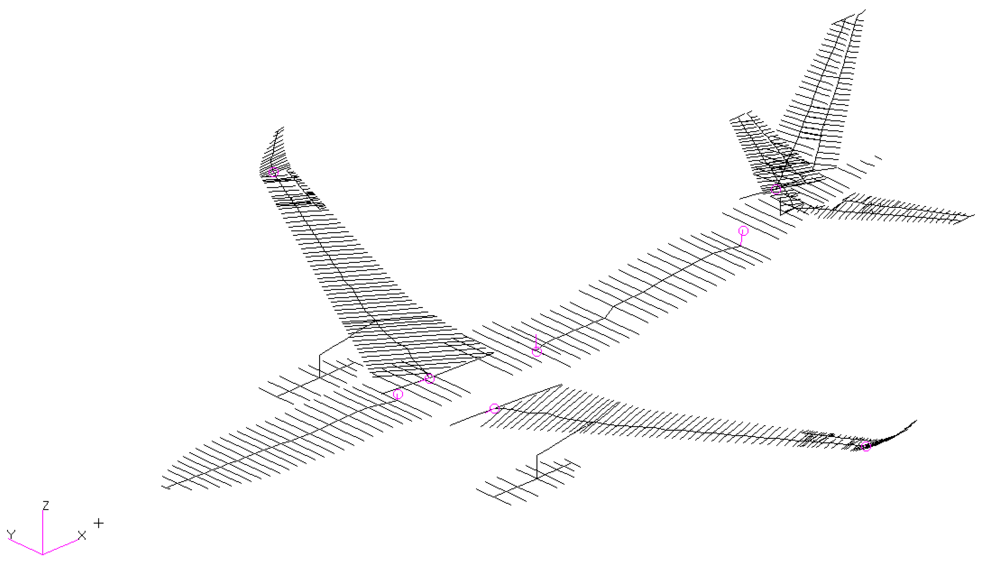
The rigid and elastic displacements of the aerodynamic model are shown in Figure 2.
3.2. Input and Output Data
The input data that affect aircraft flight loads are exceptionally complex. During different flight stages, such as takeoff, climb, cruise, descent, and landing, flight loads vary significantly. The external environment also has a significant impact on flight loads, such as the altitude, the pressure, and the wind speed. The output data, which are the load status of different components of the airplane structure, vary, and each component’s severe-load condition corresponds to different flight load conditions. Therefore, the selection of flight load conditions is crucial.
In this study, symmetric maneuver flight was used as an example for regression analysis and validation. The total weight, the center of gravity, the pitch moment of inertia, the altitude, the Mach number, the airspeed, the velocity pressure, the pitch rate, the load factor, and the angle of attack were selected as input parameters.
To comprehensively investigate the severe-load situations of various aircraft components, typical profiles of the components need to be selected, and especially wing load should be calculated to characterize load situations. In this study, the load of wing was selected as the output parameter.
3.3. Training and Test Data
The data used in this study consisting of a total of 135 sets of flight load data. Using randomization, the data were divided into a training set of 100 flight load data and a test set of 35 flight load data.
In practical engineering, the calculation of flight load often involves millions of flight load conditions. Due to limitations, this study only had 135 sets of flight load data, and it only provided a preliminary exploration of this method.
3.4. BP Modelling
The neural network used in this article was a back-propagation (BP) neural network with one hidden layer and the logistic function as the activation function. The hidden layer neuron count of the BP neural network was tuned using a loop. Figure 3 shows that the neural network had the smallest RMSE when the hidden layer neuron count was 6.
3.5. Kriging and NNRK Modelling
Given that Kriging is a very common algorithm, this section primarily introduces the modeling process of NNRK.
The so-called neural network residual Kriging (NNRK) is a process that first uses artificial neural networks to regress the results and then uses the difference between the numerical values of the actual results and the regression results of artificial neural networks as input data for Kriging. The residual of the test set is then calculated, and finally, the regression results of artificial neural networks are added to obtain the final regression result. The details of the flow chart are shown in Figure 4.
4. Result and Discussion
The BP, Kriging, NNRK results and the real loads are shown in Figure 5, Figure 6, Figure 7 and Figure 8.
From Figure 5, Figure 6, Figure 7 and Figure 8, especially the detailed diagram in Figure 7, it can be seen that the Kriging result differed the most from the actual load, while the BP result and the NNRK result were closer. It is difficult to discern which is better from the figures. It demonstrates that neural networks are more effective than Kriging in multi-parameter non-linear problems.
The MAE, the MSE, the RMSE, and the R-square are shown in Table 3.
It is clear that the regression performances of BP and NNRK were much better than that of Kriging and NNRK was slightly better than BP. This demonstrates that using Kriging to process the residuals of BP is effective and can improve the regression performance of the neural network.
Considering the small size of the data in this study, which was highly influenced by individual data, nine sets of random training and test datasets were randomly generated, and the RMSE of different methods are shown in Table 4. From the table, it can be seen that regardless of the random set, the regression of NNRK was consistently better than those of BP and Kriging, which proves that NNRK does indeed improve the results compared to the NN and Kriging.
The runtimes of three methods are shown in Table 5.
It can be observed that the runtime of NNRK was almost the same as that of the NN while Kriging had the shortest runtime.
It is worth noting that compared to the traditional CFD-CSD coupling method, which takes several tens of minutes or even several hours for each case, BP, Kriging, and NNRK were all much more efficient. In practical flight envelope calculations, using the CFD-CSD method for millions of cases would require a significant amount of computational resources. However, by incorporating neural networks or Kriging as surrogate models, the calculation time can be greatly reduced while ensuring accuracy.
5. Conclusions
This paper investigated three modeling methods for flight load regression models, namely BP, Kriging, and neural network residual Kriging (NNRK). Numerical regression results demonstrated that for multivariate nonlinear problems, neural networks have better performance than Kriging, while NNRK outperforms neural networks. This demonstrates that using Kriging to process the residuals of neural networks is very effective and time-efficient.
Overall, the flight load regression analysis based on NNRK is very effective, ensuring both computational efficiency and accuracy, and can be applied to flight load analysis.
Additionally, there is an improved version of NNRK called RKNNRK, which uses Kriging to sample at the sampling stage and then performs neural network residual regression. The data in this study is not enough to establish an RKNNRK model and compare the results. If there is an opportunity in the future, this will be studied further.
Author Contributions
Conceptualization, methodology, validation and formal analysis were conducted by Q.Y. and C.Y. investigation, resources, data curation, and writing were conducted by Q.Y. and Z.W. Funding acquisition was achieved by Z.W. and C.Y. All authors have read and agreed to the published version of the manuscript.
Funding
This research received no external funding.
Data Availability Statement
Not applicable.
Acknowledgments
Thanks are given to Dai Yuting for her guidance on this paper.
Conflicts of Interest
The authors declare no conflict of interest.
References
- Livne, E.; Weisshaar, T.A. Aeroelasticity of nonconventional airplane configurations—Past and future. J. Aircr. 2003, 40, 1047–1065. [Google Scholar] [CrossRef]
- Lee, S.J.; Im, D.K.; Kang, M.K.; Lee, I.; Kwon, J.H. Efficient Aeroelastic Analysis Method Including Inverse Design for Body Effects. J. Aircr. 2009, 46, 2164–2169. [Google Scholar] [CrossRef]
- Castellani, M.; Cooper, J.E.; Lemmens, Y. Nonlinear static aeroelasticity of high-aspect-ratio-wing aircraft by finite element and multibody methods. J. Aircr. 2017, 54, 548–560. [Google Scholar] [CrossRef] [Green Version]
- Zink, P.S.; Raveh, D.E.; Mavris, D.N. Robust structural design of an active aeroelastic wing with maneuver load inaccuracies. J. Aircr. 2004, 41, 585–593. [Google Scholar] [CrossRef]
- Rodden, W.P.; Johnson, E.H. MSC Nastran v68 Aeroelastic Analysis User’s Guide; MSC Software Corporation: Los Angeles, NY, USA, 1994; pp. 73–76. [Google Scholar]
- Venkayya, V.; Tischler, V. Force and displacement transformation for aero-structure interaction analysis. In Proceedings of the 10th AIAA/IAAMO Multidisciplinary Analysis and Optimization Conference, AIAA, Albany, NY, USA, 30 August–1 September 2004. [Google Scholar]
- Dehart, J.; Cramer, K.; Miller, S. Application of the PANAIR production code to a complex canard/wing configuration. In Proceedings of the 21st Aerospace Sciences Meeting, AIAA, Reno, NV, USA, 10–13 January 1983. [Google Scholar]
- Liu, Y.Z.; Zhu, S.Y.; Wan, Z.Q.; Yang, C. A High Efficiency Aeroelastic Analysis Method based on Rigid External Aerodynamic Force and Elastic Correction by High-Order Panel Method. In Proceedings of the 55th AIAA Aerospace Sciences Meeting, AIAA, Grapevine, TX, USA, 9–13 January 2017. [Google Scholar]
- Raveh, D.; Karpel, M. Structural optimization of flight vehicles with non-linear aerodynamic loads. In Proceedings of the 7th AIAA/USAF/NASA/ISSMO Symposium on Multidisciplinary Analysis and Optimization, AIAA, St. Louis, MO, USA, 2–4 September 1998. [Google Scholar]
- Yu, D.O.; Kwon, O.J. Predicting wind turbine blade loads and aeroelastic response using a coupled CFD-CSD method. Renew. Energy 2014, 70, 184–196. [Google Scholar] [CrossRef]
- Tang, D.; Dowell, E.H. Experimental and theoretical study on aeroelastic response of high-aspect-ratio wings. AIAA J. 2001, 39, 1430–1441. [Google Scholar] [CrossRef]
- Wan, Z.Q.; Zhang, B.C.; Yang, C.; Xu, Y. Static aeroelastic analysis of a high-aspect-ratio wing based on wind-tunnel experimental aerodynamic forces. Sci. China Technol. Sci. 2011, 54, 2716–2722. [Google Scholar] [CrossRef]
- Kutz, J.N. Deep Learning in Fluid Dynamics. J. Fluid Mech. 2017, 814, 1–4. [Google Scholar] [CrossRef] [Green Version]
- Lye, K.O.; Mishra, S.; Ray, D. Deep Learning Observables in Computational Fluid Dynamics. J. Comput. Phys. 2020, 410, 109339. [Google Scholar] [CrossRef] [Green Version]
- Halder, R.; Damodaran, M.; Khoo, B.C. Deep Learning Based Reduced Order Model for Airfoil-Gust and Aeroelastic Interaction. AIAA J. 2020, 58, 4304–4321. [Google Scholar] [CrossRef]
- Wang, X.; Kou, J.Q.; Zhang, W.W. Multi-Fidelity Surrogate Reduced-Order Modeling of Steady Flow Estimation. Int. J. Numer. Methods Fluids 2020, 92, 1826–1844. [Google Scholar] [CrossRef]
- Sun, Z.; Wang, C.; Zheng, Y.; Bai, J.; Li, Z.; Xia, Q.; Fu, Q. Non-Intrusive Reduced-Order Model for Predicting Transonic Flow with Varying Geometries. Chin. J. Aeronaut. 2020, 33, 508–519. [Google Scholar] [CrossRef]
- Ignatyev, D.; Khrabrov, A. Experimental Study and Neural Network Modeling of Aerodynamic Characteristics of Canard Aircraft at High Angles of Attack. Aerospace 2018, 5, 26. [Google Scholar] [CrossRef] [Green Version]
- Ling, J.; Kurzawski, A.; Templeton, J. Reynolds Averaged Turbulence Modelling Using Deep Neural Networks with Embedded Invariance. J. Fluid Mech. 2016, 807, 155–166. [Google Scholar] [CrossRef]
- Dong, Y.Q. An Application of Deep Neural Networks to the in-Flight Parameter Identification for Detection and Characterization of Aircraft Icing. Aerosp. Sci. Technol. 2018, 77, 34–49. [Google Scholar] [CrossRef]
- Zhang, B.; Sun, X.; Liu, S.; Deng, X. Recurrent Neural Network-Based Model Predictive Control for Multiple Unmanned Quadrotor Formation Flight. Int. J. Aerosp. Eng. 2019, 2019, 7272387. [Google Scholar] [CrossRef] [Green Version]
- Mersha, B.W.; Jansen, D.N.; Ma, H. Angle of Attack Prediction Using Recurrent Neural Networks in Flight Conditions with Faulty Sensors in the Case of F-16 Fighter Jet. Complex Intell. Syst. 2021, 9, 2599–2611. [Google Scholar] [CrossRef]
- Lee, H.; Puranik, T.G.; Fischer, O.P.; Mavris, D.N. Flight Data Driven System Identification Using Neural Networks for Landing Safety Assessment. In Proceedings of the 2021 IEEE/AIAA 40th Digital Avionics Systems Conference (DASC), San Antonio, TX, USA, 3–7 October 2021. [Google Scholar]
- Simpson, T.W.; Mistree, F. Kriging Models for Global Approximation in Simulation-Based Multidisciplinary Design Optimization. AIAA J. 2001, 39, 2233–2241. [Google Scholar] [CrossRef] [Green Version]
- Yang, L.H.; Liu, S.A.; Zhang, G.Y.; Wang, C.X. Global Optimization for Ducted Coaxial-Rotors Aircraft Based on Kriging Model and Improved Particle Swarm Optimization Algorithm. J. Cent. South Univ. 2015, 22, 1315–1323. [Google Scholar] [CrossRef]
- Gong, Q.; Zhang, J.G.; Su, D. Reliability Simulation Combining Kriging and Monte Carlo Radius-Outside Importance Sampling in Space Structure Latch. Appl. Mech. Mater. 2012, 166–169, 1872–1878. [Google Scholar] [CrossRef]
- Kanazaki, M.; Jeong, S.; Yamamoto, K. High-Lift System Optimization Based on the Kriging Model Using a High-Fidelity Flow Solver. Trans. Jpn. Soc. Aeronaut. Space Sci. 2006, 49, 169–174. [Google Scholar] [CrossRef] [Green Version]
- Ollar, J.; Mortished, C.; Jones, R.; Sienz, J.; Toropov, V. Gradient Based Hyper-Parameter Optimisation for Well Conditioned Kriging Metamodels. Struct. Multidiscip. Optim. 2016, 55, 2029–2044. [Google Scholar] [CrossRef] [Green Version]
- Lee, S.; Kang, S.; Lee, K. Development of a Gaussian Process Modeling Application for the Prediction of Missile Aerodynamic Coefficients. AIAA J. 2019, 57, 2280–2296. [Google Scholar] [CrossRef]
- Weinmeister, J.; Gao, X.; Roy, S. Analysis of a Polynomial Chaos-Kriging Metamodel for Uncertainty Quantification in Aerodynamics. AIAA J. 2019, 57, 2280–2296. [Google Scholar] [CrossRef]
- Zhou, C.C.; Ji, M.Y.; Zhao, H.D.; Fei, C. Uncertainty Analysis of Motion Error for Mechanisms and Kriging-Based Solutions. Proc. Inst. Mech. Eng. Part O-J. Risk Reliab. 2021, 235, 731–743. [Google Scholar]
- Jeong, S.; Murayama, M.; Yamamoto, K. Efficient Optimization Design Method Using Kriging Model. J. Aircr. 2005, 42, 413–420. [Google Scholar] [CrossRef] [Green Version]
- Bae, H.G.; Kwon, J.H. A Study on Constrained Efficient Global Optimization Method for Noisy Computational Fluid Dynamics Data. Proc. Inst. Mech. Eng. Part G-J. Aerosp. Eng. 2014, 228, 908–919. [Google Scholar] [CrossRef]
- Seo, Y.; Kim, S.; Singh, V.P. Estimating Spatial Precipitation Using Regression Kriging and Artificial Neural Network Residual Kriging (Rknnrk) Hybrid Approach. Water Resour. Manag. 2015, 29, 2189–2204. [Google Scholar] [CrossRef]
- Tarasov, D.; Buevich, A.; Shichkin, A.; Subbotina, I.; Tyagunov, A.; Baglaeva, E. Chromium Distribution Forecasting Using Multilayer Perceptron Neural Network and Multilayer Perceptron Residual Kriging. In Proceedings of the International Conference of Numerical Analysis and Applied Mathematics (ICNAAM 2017) 1978, Thessaloniki, Greece, 25–30 September 2017. [Google Scholar]
- Tarasov, D.A.; Buevich, A.G.; Sergeev, A.P.; Shichkin, A.V. High Variation Topsoil Pollution Forecasting in the Russian Subarctic: Using Artificial Neural Networks Combined with Residual Kriging. Appl. Geochem. 2018, 88, 188–197. [Google Scholar] [CrossRef]
- Sergeev, A.P.; Tarasov, D.A.; Buevich, A.G.; Subbotina, I.E.; Shichkin, A.V.; Sergeeva, M.V.; Lvova, O.A. High Variation Subarctic Topsoil Pollutant Concentration Prediction Using Neural Network Residual Kriging. Appl. Math. Comput. Sci. 2017, 1836, 020023. [Google Scholar]
- Shen, Z.Q.; Shi, J.B.; Wang, K.; Kong, F.S.; Bailey, J.S. Neural Network Ensemble Residual Kriging Application for Spatial Variability of Soil Properties. Pedosphere 2004, 14, 289–296. [Google Scholar]
- Demyanov, V.; Soltani, S.; Kanevski, M.; Canu, S.; Maignan, M.; Savelieva, E.; Timonin, V.; Pisarenko, V. Wavelet Analysis Residual Kriging Vs. Neural Network Residual Kriging. Stoch. Environ. Res. Risk Assess. 2001, 15, 18–32. [Google Scholar] [CrossRef] [Green Version]
- Sato, K.; Inage, K.; Fujii, T. On the Performance of Neural Network Residual Kriging in Radio Environment Mapping. IEEE Access 2019, 7, 94557–94568. [Google Scholar] [CrossRef]
- Angiulli, G.; De Carlo, D.; Sgró, A.; Versaci, M.; Morabito, F.C. Accurate Modelling of Lossy Siw Resonators Using a Neural Network Residual Kriging Approach. IEICE Electron. Express 2017, 14, 20170073. [Google Scholar] [CrossRef] [Green Version]
Figure 1.
Structure model of the plane.

Figure 2.
Rigid and elastic displacements of the aerodynamic model. (The pink color represents the rigid displacement; the green represents the elastic displacement; the blue color represents the original model).
Figure 2.
Rigid and elastic displacements of the aerodynamic model. (The pink color represents the rigid displacement; the green represents the elastic displacement; the blue color represents the original model).

Figure 3.
RMSEs for different neuron counts.

Figure 4.
Flow chart of neural network residual Kriging.

Figure 5.
Wing loads of different methods.

Figure 6.
Comparison between the real load and the regression load.

Figure 7.
Detailed comparison between the real load and the regression load. (a) Detailed comparison; (b) Detailed comparison.
Figure 7.
Detailed comparison between the real load and the regression load. (a) Detailed comparison; (b) Detailed comparison.


Figure 8.
Relative errors of different methods.


Table 1.
Input parameters.
| Meaning | Unit |
|---|---|
| Total weight | kg |
| Center of gravity | % |
| Pitch moment of inertia | kg × m2 |
| Altitude | m |
| Mach number | Non-dimensional |
| Airspeed | m/s |
| Velocity pressure | pa |
| Pitch rate | |
| Load factor | Non-dimensional |
| Angle of attack |
Table 2.
Output parameter.
| Meaning | Unit |
|---|---|
| Wing load | N |
Table 3.
Numerical comparison between different methods.
| BP | Kriging | NNRK | |
|---|---|---|---|
| MAE | 0.020730 | 0.112119 | 0.016246 |
| MSE | 0.000648 | 0.065690 | 0.000575 |
| RMSE | 0.025456 | 0.256301 | 0.023981 |
| R-square | 0.999790 | 0.982193 | 0.999820 |
Table 4.
Comparison of the RMSEs for different methods of random datasets.
| BP | Kriging | NNRK | |
|---|---|---|---|
| Random dataset 1 | 0.050018 | 0.746040 | 0.027682 |
| Random dataset 2 | 0.028923 | 0.935631 | 0.024446 |
| Random dataset 3 | 0.160216 | 1.041563 | 0.040264 |
| Random dataset 4 | 0.036385 | 0.101322 | 0.025585 |
| Random dataset 5 | 0.044994 | 0.071680 | 0.030333 |
| Random dataset 6 | 0.034482 | 0.081201 | 0.019517 |
| Random dataset 7 | 0.078744 | 0.844058 | 0.018788 |
| Random dataset 8 | 0.067317 | 1.399952 | 0.060299 |
| Random dataset 9 | 0.057461 | 0.054945 | 0.053900 |
Table 5.
Runtimes of different methods.
| BP | Kriging | NNRK | |
|---|---|---|---|
| Time (s) | 1.31 | 0.078 | 1.34 |
Disclaimer/Publisher’s Note: The statements, opinions and data contained in all publications are solely those of the individual author(s) and contributor(s) and not of MDPI and/or the editor(s). MDPI and/or the editor(s) disclaim responsibility for any injury to people or property resulting from any ideas, methods, instructions or products referred to in the content. |
© 2023 by the authors. Licensee MDPI, Basel, Switzerland. This article is an open access article distributed under the terms and conditions of the Creative Commons Attribution (CC BY) license (https://creativecommons.org/licenses/by/4.0/).
Share and Cite
MDPI and ACS Style
Yan, Q.; Wan, Z.; Yang, C. Flight Load Calculation Using Neural Network Residual Kriging. Aerospace 2023, 10, 599. https://doi.org/10.3390/aerospace10070599
AMA Style
Yan Q, Wan Z, Yang C. Flight Load Calculation Using Neural Network Residual Kriging. Aerospace. 2023; 10(7):599. https://doi.org/10.3390/aerospace10070599
Chicago/Turabian StyleYan, Qi, Zhiqiang Wan, and Chao Yang. 2023. "Flight Load Calculation Using Neural Network Residual Kriging" Aerospace 10, no. 7: 599. https://doi.org/10.3390/aerospace10070599
Note that from the first issue of 2016, this journal uses article numbers instead of page numbers. See further details here.