
Fiber Optic Ice Sensor for Measuring Ice Thickness, Type and the Freezing Fraction on Aircraft Wings

Physics Department, University of Ioannina, 45100 Ioannina, Greece
Aerospace 2023, 10(1), 31; https://doi.org/10.3390/aerospace10010031
Submission received: 24 October 2022
/
Revised: 25 December 2022
/
Accepted: 27 December 2022
/
Published: 30 December 2022
(This article belongs to the Special Issue Deicing and Anti-Icing of Aircraft (Volume III))
Abstract
:Ice accretion on an aircraft affects the aerodynamic performance of the wings by disrupting the airflow, increasing drag, and altering its flight characteristics, leading to a main or tail wing-stall and altimetry to aircraft loss. The current generation of ice-detection systems relies on environmental parameters to determine icing conditions, with the sensors usually located on the nose of the aircraft, giving no information on the ice accreted on the wings. This work focuses on modeling and developing a fiber-optic-array ice sensor, which illuminates and detects the reflected and scattered light directly from the ice surface and volume, and measures the accretion rate and type of ice on the wings. The ice morphology is influenced by the rate of freezing of the super-cooled droplets impacting the wings, and partially or totally trapping the dissolved gasses. This leads to the formation of rugged surfaces and ice shapes, which can be transparent or opaque, a process which is dependent on the local Freezing Fraction (FF) of the impinging super cooled water. The detection method relies on the optical characteristics of ice, affected by density and the size of micro-cracks and micro-bubbles formed during freezing. By using high Numerical Aperture (NA) fibers, it was possible to accurately measure the ice thickness, and to investigate a proof-of-concept experiment, correlating the optical diffusion to the FF of the ice on a wing.
1. Introduction
The phenomenon of icing in aviation is a complex atmospheric condition, which occurs when an aircraft flies through cold moist air, resulting in ice accumulation on the wings. This increases drag, reduces lift, and can potentially lead to a stall. It is particularly dangerous during take-offs and landings, or when aircrafts are in low-level holding patterns near airports and fly through freezing fog. Usually, ice accretes on the leading edge of wings, growing forward into the air stream with a morphology which is determined by the ambient conditions, airspeed, and aerodynamics of the wing. Although icing is a rare phenomenon, occurring in only 3% to 5% of the flight envelopes, there are a number of reported accidents which have involved ice protected aircrafts, indicating there are inadequacies in the current generation of ice detection and protection systems [1,2]. As a result, there is ongoing interest and research focused on developing ice detection and protection technologies for the aviation industry. The first ice sensors were introduced in 1956 in military aviation, using a pressure difference that changed if ice was detected. Subsequently, a number of ice sensors were developed for commercial aviation using vibrating surfaces, heat of fusion, rotating cylinders, ultrasonic, dielectrics, microwaves, acoustic and optical polarization [3].
Current ice sensors use either direct or indirect methods to determine the presence of ice, and are usually point-sensors located on the nose or the fuselage of the aircraft. Direct sensors detect ice accretion using either a hot wire, to measure the energy required to keep the wire ice free [4], or vibration elements that alter the resonant frequency by the accreted ice mass [5]. These types of sensors work cyclically, as they need to shed the ice prior to initiating a new measurement cycle. Conversely, indirect sensors usually measure atmospheric conditions such as humidity, liquid water content (LWC), and ambient temperature, to determine icing conditions based on algorithms [6]. However, contemporary ice sensors’ architectures cannot detect the presence, type, or accretion rate of ice on critical lift areas, such as the main wings or tail stabilizer wings, which have different “tolerances” for ice, and can affect the handling characteristics of the aircraft differently. Important parameters in ice detection are the response time and duty-cycle of the ice sensors, which due to the cyclic nature of the measurements can be slow. This can be a problem in severe icing conditions such as with Super Large Droplet (SLD) ice, and can potentially overload the ice protection system. Another area of concern is engine icing due to high altitudes’ ice-crystals, causing a loss of power (rollback) without any warning, and being undetectable by current generation ice sensors [7]. Engine icing, related to high altitude crystals, is a relatively new discovery that is currently adopted by the research community and the aviation industry [8]. As a result of these inadequacies, the FAA and other aviation regulatory authorities have proposed new rules regarding ice protection systems which include SLD and high-altitude ice crystal detection [9]. Furthermore, new technologies have been researched using direct or indirect ice detection systems, located on the aerodynamic surfaces, or relying on data from the sensors in the aircraft to indirectly detect icing conditions and severity.
Some of the current studies on direct ice point-detection systems employ piezoelectric actuators with variable natural frequency with ice growing, followed by melting to begin a new measurement cycle [10]. Another similar approach uses silicon micro-wafer diaphragm-actuators, whose characteristic stiffness is altered by the accreted ice [11]. Another direct ice detection scheme is based on surface acoustic “love-waves” propagating on the wing skin, detecting ice as a change in the traveling wave on wings [12]. A recently developed sensor exploits the variations in dielectric properties of ice and water (εw, ει), which alters the spectral characteristics and resonant frequencies of a split ring resonator sensor, located on the aerodynamic surfaces [13,14]. Another approach is to use energy self-sustaining, wireless detection sensors, located on the outer surfaces of the aircraft, to detect the presence of ice by the change in the surface capacitance due to the presence of ice [15]. However, these sensors can only detect the presence of ice, but cannot provide information on its type, ice thickness, or rate of accretion, nor are they capable of distinguishing Super Large Droplets (SLD) ice, which results from large sized droplets which can splash-back and refreeze in unprotected areas of the wing. Similarly, some indirect experimental ice detection systems rely on “smart” algorithms, using flight data from the aircraft systems to detect changes in the flight characteristics of the aircraft, such as drag, lift, and engine power, instigated by ice accretion [16]. Engine icing, on the other hand, involves ice crystals in the range of 2 μm to about 200 μm, which are elevated to high altitudes by updrafts following tropical storms, and are inhaled by jet engines, melting and refreezing in the low compression stages of the engine. This ice disrupts the airflow, resulting in loss of power (rollback), and can lead to overheating and engine damage. Moreover, conventional ice sensors cannot detect ice crystals, as they do not accrete ice except inside the engines, requiring the development of bespoke engine ice sensors located inside the turbine [11,12].
To overcome some of the current generation ice sensors’ shortcomings, new direct ice detection approaches have been proposed using the electrostatic [13,14,15], as well as the optical properties of the ice to detect it directly on critical areas of the wings or the engine. In previous work, we reported on a fiber optic array ice-sensor located on the stagnation line of the wing, which can measure in real time the rate of accretion, thickness, and its type of ice, using optical diffusion in ice [17]. In another similar approach, researchers have used an angled fiber-bundle sensor to detect the ice presence and thickness [18]. Fiber Bragg Gratings, which can respond very rapidly to changes in temperatures, have also been used to detect ice through the variations in temperature caused by the latten heat of freezing [19]. Generally, the rate of growth and shape of the ice accreted on the airfoil is dependent on the airspeed, LWC, temperature, wing aerodynamics, and droplet sizes or mean volume diameter (MVD), and is broadly classified in glazed, rime, or mixed phase ice, with each type having distinct morphology and optical characteristics.
A key parameter, which determines the ice accretion process on aerodynamic surfaces, is Messinger’s Freezing Fraction (FF), defined as the ratio of the super-cooled droplets that freeze on impact, together with those which remain liquid in a given volume. It is a dimensionless quantity with values ranging from 0 to 1 [20]. It is used primarily as a modeling tool for aircraft wing and de-icing system development, as well as in algorithms that assess ice severity condition. Glazed ice, for instance, is accreted at near freezing temperatures, −3 °C to −5 °C, and has low FF values (0.1 to 0.3); this gives clear transparent ice, as the droplets partially freeze on impact, and the dissolved gasses in the super-cooled droplets can escape. Conversely, at lower temperatures of −20 °C and below, the FF is close to 1 and the super-cooled droplet totally freezes on impact so the dissolved gases cannot escape, forming high concentrations of micro-bubbles, and accretion of rime ice with its characteristic white opaque appearance [20,21]. It is therefore important to distinguish the different types of ice on the wings, and how they affect the flight characteristics of the aircraft. Glazed ice, for instance, has a rough and rugged surface which grows above and below the leading edge of the wing, disrupting the airflow, as shown in Figure 1a,b. Rime ice, on the other hand, is smoother, usually extending forward from the leading edge of the wing, and it is less disruptive to the airflow. Knowledge of ice-type could potentially be useful for smart-zone de-icing systems, which have the capability to alter the de-icing sequences, reducing power consumption. Furthermore, the freezing process inadvertently affects the value of the FF, as well as the optical characteristics of the different types of ice, by altering the concentrations of micro-bubbles and micro-cracks, and this interdependence is addressed in this paper. It should also be noted that, at present, there is no easy direct method to measure the FF on the wing of an aircraft, as there is no access to relevant ice parameters.
If an optical ice detector could measure the accretion rate, ice thickness, as well as the FF on wings in real time, it could provide additional valuable information of the ice severity, enhancing aircraft safety. Therefore, one of the aims of this work is to investigate the relation of the optic parameters with ice thickness and type, and correlate the optical diffusion process with the FF fraction based on Messinge relation [20], and used by Anderson and Tsao in NASA-Glen [22]. As will be discussed in more detail in Section 5, it is suggested that the reflected and scattered light for different types of ice, which have discrete optical signatures, can potentially be calibrated to the corresponding FF value, thus linking these two parameters.
In this work, a Fiber Optic Array Ice Sensor (FOAIS) was developed, optimized, and used to investigate the optical characteristics of ice accreting on the leading edge of a wing in an icing tunnel. The ice sensor illuminates the ice, from inside the wing through a window, and detects scattered and reflected light from the micro-bubbles and the ice surfaces, obtaining unique optical intensity “signatures” which are effectively the optical diffusion, for the different types of ice accreting on the wing. Through calibrations, the optical signatures can be used as a proof-of-concept to determine the ice thickness and type by measuring the relative reflection and scattering contributions to the detected signals. Furthermore, both the FF and optical diffusion in ice are directly affected by the icing conditions, and seem to be interdependent. To assess their connection, we modeled the optical intensities, optimizing the ice sensor geometry and correlating the FF to the characteristic optical diffusion signatures. The work was conducted at GKN aerospace research icing tunnel in the UK, which was calibrated using a NACA 0012 wing, giving very similar ice shapes to those of the NASA-Glenn facility which was used by [22].
2. Materials and Methods
2.1. Optical Diffusion in Ice and Sensor Configuration
An optical beam, illuminating the ice from inside the wing, will partially scatter from the micro-bubble discontinuities and diffuse in the ice volume, with the remaining light undergoing specular reflections from the rugged ice surfaces [23]. Ice formed on the wing at temperatures close to freezing (−1 °C to −5 °C) is glazed with a low FF value, and a large percentage of the water remains unfrozen, running-back and refreezing on cooler regions of the wing. This mechanism forms secondary ice at the impact point, generating ragged, near-transparent surfaces with distinctive shapes and “horns” or “feathers”, which are particularly disruptive to the airflow, as shown in Figure 1a, and its cross-section in Figure 1b [2]. At lower temperatures of −20 °C and below, all the water in the super-cooled droplet freezes on impact, having an FF value close to unity. The accreted rime ice is smooth, with a characteristic white opaque appearance, attributed to rapid freezing and the trapping of the dissolved gasses in the ice volume, as shown in Figure 1e,f. In intermediate conditions, −10 °C to −15 °C, the temperature over the wing can vary in a way that the ice accreted on the stagnation line could be glazed, while over the top and bottom surfaces, were the air accelerates and cools, it accretes near opaque ice known as mixed phase ice (Figure 1c,d).
2.2. Principles of Ice Detection with Fiber Optic Array Sensor
The principle of optical ice detection relies on measuring the optical characteristics of the different types of ice as it accretes, using a fiber-array sensor located on the stagnation line behind a window on the leading edge of the wing, which illuminates and detects light from the ice as shown in Figure 2a–c. The accreting ice is illuminated by the central, illumination fiber of the FOAIS, and depending on the ice type, some of the light is scattered by the trapped micro-bubbles and micro-cracks in the ice volume, while the remaining is partially reflected at the ice–air interface, and the rest is transmitted out of the ice volume. This light is detected by the signal or detection fibers, situated symmetrically on either side of the illumination fiber, as shown schematically in Figure 3a. Therefore, the key parameters which influence the optical response of the FOAIS are the concentration of the scattering centers in the ice, and the surface morphology of the ice–air interface, both of which are directly related to the way ice is formed, hence its FF.
Other important parameters are the fiber optic geometry, such as inter-fiber separation and the source and signal fibers NA, which determines the illumination beam divergence, and the detection angles of the signal fibers, respectively. According to Snell’s law, the divergence of the illumination beam and the acceptance angles of the fibers are dependent on the refractive index, m of ice and the optical diffusion of the narrow beam, which is depended on the concentration and size of the scattering centers in the ice volume. As ice does not absorb light in the visible spectrum, and the size of the trapped bubbles and micro cracks are equivalent to optical wavelengths (350 nm to 850 nm), Mie scattering is the dominant diffusion mechanism giving the ice a white appearance [24]. The signal fibers will thus detect backscattered and reflected light, which falls within their acceptance cone (NA), and the intensity will vary with increasing ice thickness from which the characteristic optical diffusion curves are taken.
2.3. Background of Fiber Optic Ice Sensor Modeling
Based on the above, if we consider the onset of semi-transparent ice, the ragged air–ice interface is initially near the sensor as the ice is very thin, and will thus couple a small percentage of reflected light into the detection fibers, while the scattering signals are low due to the low illumination volume. With increasing ice thickness, however, more of the ice volume is illuminated with a corresponding increase in the scattering signals, while the reflected contributions decrease as the ice surface is retreating away from the detection fibers. The optical contributions of these two mechanisms are directly affected by the surface morphology and density of the scatterers. Therefore, the relative intensity contributions from specular surface reflections and scattering can be modeled separately by considering the illumination process, and the way the light couples into the signal fibers for the different types of ice.
2.3.1. Reflection Contributions
The reflection contributions can be modeled by the overlap of the illumination and detection regions projected on the ice–air interface, which increases with ice thickness, increasing the reflected light which falls within the acceptance angle of the signal fibers, as shown schematically in Figure 3a. However, as the ice thickness x increases, the ice–air interface progressively retreats away from the detection-fibers, and the intensity Ix reduces, obeying to a good approximation the inverse square i.e., Ix = I0/x2. As will be shown experimentally and in the simulations, the overall effect for the inner fibers is an initial gradual increase in intensity, reaching a maximum when the ice thickness is such that the ice–air interface reflects nearly all the light within the acceptance angle of the signal fibers. However, as the ice thickness increases, and the ice–air interface retreats away, reflections fall outside the acceptance angles of the fibers, resulting in a progressive reduction in intensity. Therefore, in a first principles approximation, the detected light by the signal fibers can be modeled as the overlap area (Aoverlap (x)) of the illumination and detection circles, which expand with increasing ice thickness, x given as:
where a is the fiber acceptance angle in ice, calculated from the fiber NA, d is the source/signal fiber separations, and r(x) is the radius of the overlapping circles on the air/ice surface Figure 3b. Furthermore, the peak intensity I0 obeys Fresnel reflection criteria, i.e., the reflection intensity at the interface is about 4% of the incident intensity I0 and due to ragged ice surfaces, the specular reflections obey cosine angular distribution given as
where φ is the specular reflection angle, as shown schematically in Figure 3b. In opaque ice, the beam scatters, reducing the reflection contributions reaching the fibers. However, it was observed that even in white rime ice, there was always a small reflection, as is discussed below.
I(φ) = I0 cos(φ)
2.3.2. Scattering Contributions
As outlined above, in addition to specular reflections, the presence and concentration of the micro-bubbles and micro-cracks in the ice will scatter the beam, diffusing light in the ice volume. In general, when the wavelength of the light is comparable to the size of the scatterers, shorter wavelengths are scattered more than longer ones (Iscattering ∝ λ−4). These scatter in all directions, perpendicular to the polarization of the light, with a “donate-like” spatial distribution known as Rayleigh scattering. Conversely, when the scatterers are larger than the wavelength of the light, all wavelengths are scattered equally (Iscattering ∝ λ), mostly in the direction of light propagation or forward direction, known as Mie scattering [24]. Therefore, for rime white ice accreted on aerodynamic surfaces (Figure 1e,f), Mie scattering is the dominant mechanism [24]. As scattering is a complex process, a full analysis is beyond the scope of this work, but to aid modeling the detected signals, a brief outline is given below. It can thus be simplified as a macroscopic process, based on the Beer Lambert law applied to a collimated beam, given as:
where the initial intensity I0 is attenuated in the ice of thickness x. In Equation (3) μs is the reduced scattering coefficient, given as μs = ρs σs, where ρs is the number density of the scattering media, σs is the effective cross-section area of scatterers. Depending on the wavelength λ and the size of the scatterers, a collimated unpolarized beam will scatter light at an average angel θ to the beam propagation, determined by the scattering anisotropy g1 given as:
and having values from 0 to 1. For g1 = 0, scattering is isotropic which is the case for Rayleigh, giving an omni-directional “doughnut”-like average angular distribution. For g1 close to 1, Mie scattering is observed, which scatters light anisotropically in the forward direction [24]. It is interesting to note that the g1 parameter will determine the optical diffusion of the beam in the media, and this point will be addressed later. Thus, the reduced scattering coefficient μs can be expressed as:
where λref is related to a reference wavelength in the visible (500 nm for instance), fRay and fMie are constants related to scattering cross sections, and b has values from 0.3 to 1 depending on the scattering medium [23,24]. Therefore, at the onset of icing when the ice is thin, most of the illumination beam is transmitted though the ice with low scattering, and hence low signals on the detection fibers. For rime ice Mie scattering dominants so relation (5) can be reduced to:
g1 = <cos(θ)>
Incorporating backscattering in the model involves calculating the increase in backscattered light as a function of ice thickness x using the Beer-Lambert law (3), as:
Therefore, if there is no ice present there will be no signal, but with increasing ice thickness, more light is backscattered and diffuses in the ice volume. This increases the detected signals which eventually reach a maximum, determined by the density of the scattering centers ρs in the ice. The total optical power, for each of the signal fibers in FOAIS, was modeled by the addition of the reflections and backscattered contributions as a function of ice thickness, generating characteristic curves for the different types of ice, which are discussed in Section 4.
2.3.3. Freezing Fraction Parameter
Ice accretion on aerodynamic surfaces is a crystal-forming process, which can take numerous forms and shapes depending on air speed, LWC, ambient temperature, MVD of the droplets, and airfoil aerodynamics. In general, air accelerates over the top and bottom of the wing, expanding adiabatically, and cools, while on the stagnation line it is compressed and heats up, forming a temperature gradient over its wing surface. Super-cooled droplets partially or totally freeze on impact giving up their latent heat of fusion, further modulating the surrounding air temperatures over the wing, accreting different types of ice over its surface [2,24]. The ice is generally irregular, with a rugged morphology, depending on the local conditions over the wing. The FF is a very useful parameter, primarily for modeling the ice thickness and shapes forming on the wings of the aircraft. It is determined by the ratio of partial or total droplet freeze on impact, which invariably affects the percentage of the dissolved gases trapped in the ice volume, modifying the surface morphology and micro-bubble concentration in the ice volume [20,22]. This, in turn, will modulate the way light interacts and diffuses in the ice volume giving it its unique optical characteristic. The above mechanism can be summarized as a set of interacting heat losses and gain processes, described in more detail Messinger’s paper [20] as a net rate heat flow q given as
and used in the derivation of the FF. In the above relation, fc is the unit convection conductance, A is the surface area, ts is the equilibrium surface temperature, is the ambient free-stream temperature, and r is the recovery factor applying to kinetic heating. is the free-stream velocity, g is the gravitational constant, cp and cw are the unit heat capacity of air and water, respectively, Rw is the unit rate of water catch by the wing, and J is the mechanical equivalent of heat.
Anderson and Tsao, Ref [22], used Messinger’s relations to calculate the FF for a neutral lift airfoil, NACA 0012, in the NASA-Glenn icing tunnel at the stagnation line of a wing. The FF, or (n) in this context, can be defined more rigorously as the fraction of water flux entering a known volume, which freezes in this volume and is given as
In the above relation, Δ is the ice thickness, d is leading edge diameter of the wing in cm, the FF is denoted as n, and Ac is the accumulation parameter, given as
and β0 is the collection efficiency of ice at the stagnation line, both being dimensionless parameters. In the above equation LWC, V, are, respectively, the Liquid Water Content and airspeed in m/s, τ is the icing run duration time in minutes, and ρ is the ice density in g/m3. According to Anderson and Tsao [22], the estimated uncertainties in their experiments for LWC were about 12%, giving corresponding n uncertainty of about 15%. Relations (9) and (10) will be used in the calculation of the FF using MS Excel, and are discussed in more detail in Section 5.2.
3. Ice Sensor Lay Out and Experimental Setup
As outlined in Section 2.1, the FOAIS encompasses a central illumination, or source fiber, which transmits light from a diode laser to the ice, and six detection, or signal fibers, situated symmetrically either side of the source fiber, couple light from the ice to a detection unit, as shown in Figure 2c and Figure 4a. The fiber-array sensor has a total active area of about 8 mm and is located inside the wing, about 1 mm behind a sealed protection glass window, so as to avoid Fresnel reflections from its inner and outer surfaces reaching the signal fibers (Figure 3b). The protection window was flush mounted on the stagnation line of the wing so it did not interfere with the ice accretion process, as shown in Figure 2c. In the experiments, several wavelengths were used, ranging from 530 nm, 650 nm, 532 nm, and 830 nm. Both the source and signal fibers were Multi Mode (MM), with a silica core and polymer cladding, having 200 μm outer diameters and 20 μm cladding with a Numerical Aperture of 0.35 to 0.45. In some experiments, however, plastic optic fiber tapers were used with a much wider effective NA of 0.7 to reduce optic noise emanating from spurious reflections on the surface of the accreting ice.
The icing tunnel had a cross section of 76 cm width by 51 cm height, with two heated side-observation windows used for independent measurements of the ice thickness during icing runs, as shown in Figure 4a–c. Several wings were used in the experiments, but for the comparison study with [22], this wing had a cord of 31 cm and was placed vertically in the icing tunnel, with the FOAIS being situated at the center of the tunnel. The signals from the fiber array were detected by corresponding photodiodes, and processed by a Data Acquisition System (DAS), consisting of individual channels, one for each fiber, which digitized and stored the data in a computer using a Labview environment. The results obtained for each fiber of the array corresponded to the variations of the optical intensity as a function of increasing ice thickness, giving a unique set of traces for each type of ice.
To enable FOAIS to measure ice thickness accreted on wings, it was calibrated in the icing tunnel by measuring the actual ice thickness independently, in real time, using an optical shadowgraph setup. It comprised a flat collimated laser beam, formed by a system of cylindrical lenses, and projected through one of the observation windows of the icing tunnel. It was aligned perpendicularly to the leading edge of the wing, passing near the fiber-optic array sensor. The beam was detected on the opposite side-window by a flat, horizontal fiber-array, consisting of about 50 fibers with 250 μm OD, aligned adjacently to each other on a substrate. The other end of the flat fiber array formed a circular fiber bubble which coupled the light to a single detector, measuring the collective optical intensity from all the fibers, as shown in Figure 4a,c. As the ice accretes on the stagnation line of the wing, the flat beam is obscured, reducing the optical intensity which was calibrated as a function of ice thickness. This arrangement was capable of detecting ice up to 12.5 mm thick, with an accuracy of about 2% to 3%, on the leading edge of the wing. The shadowgraph was used for calibration in all the icing tunnel runs to calibrate the optical diffusion curves generated by the fiber array sensor, as will be outlined in the experimental procedure in Section 5.1. An additional function of the shadowgraph laser beam was to monitor the density of the cloud. This was achieved by monitoring the brightness of the beam as it transverses the cloud inside the tunnel by imaging the forward scattering light. As shown in Figure 4c, the beam is only visible in the presence of the cloud, and by suitable imaging of the beam on a photo-detector of an optical power meter, it is possible to obtain qualitative and quantitative information from the cloud. Specifically, with the axis of the optical setup at an angle of about 25° to 30° above the plane of the beam, the signal detected by the power meter is directly proportional to the density of the cloud, which is related to the droplet size, and LWC. Although this was used only as a qualitative procedure performed in the beginning of testing runs, it was sufficient for monitoring the cloud distribution in the vicinity of the fiber array sensor.
4. Modeling the Response the Fiber Sensor Array and Freezing Fraction
As outlined in Section 2, modeling the optical intensities measured by the signal fibers, for different types of ice, relies on the overlap of the illumination and acceptance cones inside the ice volume, as shown in Figure 3b. For glazed ice, which has low scattering contributions, the signals are predominantly due to specular reflections of the beam and were modeled as Lambertian diffuse reflections from the rough ice–air interface, with an angular dependence of I = I0 cos(φ) (2). If the detected intensity for ice of thickness x, at the signal fibers is Ix, it can be assumed that it obeys, to a good approximation, the inverse square i.e., Ix = I0/x2. For mixed-phase and rime ice, scattering becomes significant, and the fibers additionally detect the backscattered light, which falls within their acceptance angles. Consequently, the intensities for the inner fibers are higher due to the close proximity to the source fiber. However, it should be noted that due to the randomness of the ice accretion process, modeling can only give an indication of the average expected signals with ice thickness.
For practical reasons, all the fibers had the same NA of 0.43 to 0.45, with the six signal fibers, designated as 1 to 6, and arranged with three on either side of the illumination fiber, which was located in between fiber 3 and 4 with an inter-fiber separation of 1 mm, as shown in Figure 3a. The modeled output power of the source fiber was set to 1 mW of monochromatic light. These parameters were simulated using inverse square law and relations (1), (2), and (7), for clear, glazed rime ice, to determine the intensity contributions to each of the signal fibers as a function of ice thicknesses x. Typical simulations using Excel, for glazed, mixed-phase, and rime ice for fiber 4 (located adjacent to the source fiber), are shown Figure 5a–c, respectively. In these Figures, the reflected, backscattered, and the total combined intensities are shown in black, red, and blue traces, respectively. Specifically, Figure 5a shows the simulation for transparent, low scattering glazed ice, while Figure 5b shows the calculated signals for mixed phase ice with significant scattering contributions to the overall signal. Finally, Figure 5c shows that for rime ice, scattering is the dominant signal.
Additionally, the detected intensities for one side of the sensor array were modeled, i.e., signal fibers 4, 5, 6, for glazed and mixed-phase ice, and the results are shown in Figure 6a,b. In these simulations, the signal fibers were also separated from the source fiber by 1 mm, 2 mm, and 3 mm, respectively, with the illumination fiber in between fiber 3 and 4, also separated by 1 mm from each other, and an illumination intensity of 1 mW. As it can be seen from these results, in the case of glazed ice in Figure 6a, all three fibers have an initial increase in intensity, attributed to the reflection contributions coupling in the fibers, which peak at the first 3 mm to 4 mm of ice growth. As expected, the reflection is more intense for the inner fiber 4, located closest to the source fiber, detecting both the reflected and scattered light. Conversely, fibers further away exhibit lower peak intensities, with fiber 6 having a smooth transition without a peak, as the reflection contributions are progressively lower and are detecting mostly scattered light. An interesting prediction of the model is the effect of the fiber NA, and the distance of the FOAIS from the protection window, which determines the minimum ice thickness detected by each of the fibers. Both these parameters should be optimized so the overlaps of the illumination and detection cones are near the window’s outer surface to avoid “blind spots” during the onset of icing, i.e., when the ice is very thin. Similarly, for near rime ice shown in Figure 5b, the traces for the three fibers do not show a distinct reflection peak, as scattering becomes dominant with increasing ice thickness. Therefore, the predicted minimum ice thickness which each of the three fibers can detect, indicated by the zero signals at the onset of icing, seems to be reduced for the outer fibers, and is directly dependent on the array geometry, location of the window, and the NA of the illumination and detection fibers. Therefore, the above parameters should be optimized when designing FOAIS.
One observation from the model is that in glazed ice, where scattering contributions are low and reflections dominate, the inner signal fibers closest to the source fiber detected the strongest signals, which increase from zero ice thickness, peaking at around 3 to 4 mm of ice. This is to be expected as the specular reflections from ice–air interface gradually align with the acceptance angle of the fiber, reaching a maximum which subsequently reduces as the ice surface retreats away from the optimum position. At greater ice thickness, the detected signals emanate from diffused scattered light, resulting in a reduction in the signals, eventually reaching a constant level. Scattering, on the other hand, is the dominant signal contributor to the outer fibers, which exhibit a lower and gradual increase in intensity, reaching a constant level with increasing thicknesses. In conclusion, the model predicts that the relative intensity of reflected and backscattered signals for the fibers in the array are dependent on the geometry of the sensor array, the morphology of the ice surface, and the density of the micro-scatters in the ice, which change with the type of ice. This is an important point which will be utilized for the measurements by the array of very thin ice (onset of icing) using the inner fibers for ice up to 3 mm thick, and using the outer fibers for greater ice thicknesses of 7 mm to 10 mm. Another important point is that the model could be used to determine the relative reflection and scattering intensity contributions for the different types of ice accretes, and then correlated to a corresponding FF value, as will be outlined in the following section.
5. Icing Tunnel Experimental Results and Discussion
5.1. Shadowgraph Calibration Procedure and Results
For the FOAIS to measure ice thickness accurately on the stagnation line of a wing, it is required to be calibrated using the aforementioned shadowgraph technique. Therefore, as described in Section 3, the ice thickness was measured accurately using the shadowgraph technique at the leading edge of the wing through the observation windows of the icing tunnel, as shown in Figure 4a,c. As the shadowgraph beam was interrupted by the accreting ice, reducing the optical signal, it was possible to measure accurately the ice thickness, as shown in Figure 7. In this figure, the black trace is the reduction in intensity with ice thickness Ix, while the black trace is, for convenience, the maximum intensity with no ice x = 0 (I0) from which Ix is subtracted i.e., I = (I0 − Ix). In this way, the optical intensities from each of the six fibers of the FOAIS, which detected the ice growth from inside the wing, as shown in Figure 8a and Figure 9a,b, could be calibrated by using the shadowgraph measurements. Furthermore, the intensity and shape of the flat beam could be adjusted as required to improve the accuracy of the calibration’s procedure for the inner and outer fibers, and is discussed in the following section.
5.2. Icing Tunnel Experiments and Calibrations
Using the experimental set up shown in Figure 2b, glazed, mixed phase, and rime ice were accreted on the wing, at icing tunnel temperatures ranging from −5 °C to −25 °C, with LWC of about 1 gm/m3. The size of the water droplets in the “cloud” had a MVD of about 20 μm, and the air speed was set at 150 knots with source-fiber output power set at 1 mW to 2 mW. These values were chosen to be similar to those used in [22]. Figure 8a shows typical ice growth curves of the intensity variations for each of the six fibers with ice thickness, as measured by the shadowgraph. This figure shows, in effect, the optical diffusion curves for glazed ice accreted for temperatures −3 °C to −5 °C. The source fiber is invariably located in the center of the array, in between fibers 3 and 4, with each of the traces corresponding to signals from the individual fibers of the ice sensor. Figure 8b displays pictures of a typical icing run, showing increasing ice thickness together with the corresponding signals, detected by the DAS, during the initial phases of the ice growth process.
Figure 9 shows comparative ice growth curves from the FOAIS for glazed ice accreted at −3 °C to −5 °C (Figure 9a), mixed phase ice accreted at −7 °C to −13 °C (Figure 9b), nearly rime ice accreted at −15 to −20 °C (Figure 9c), and totally rime ice accreted at −25 °C (Figure 9d). Usually, the morphology of glazed is rugged, growing outward into the airflow generating “horns” on the upper and lower surfaces of the wing, as seen in Figure 1a,b, and is particularly disruptive to the airflow. This is due to the adiabatic expansion and cooling of the air flowing over and under the stagnation line of the wing, increasing ice accretion in these areas. In this type of ice, the dissolved gasses in the droplets can escape, giving nearly transparent ice with low concentrations of micro-bubbles and micro-cracks, as seen in Figure 1a,b and Figure 9a. For this transparent ice, the signals from the fibers 2, 3, 4, and 5, located closer to the source fiber, detect the reflected light, which is manifested as an initial increase in intensity, peaking at ice thicknesses of 2 mm to 3 mm due to light falling within optimum acceptance angle of these fibers (Figure 9a). With greater thickness, the reflecting ice–air inter-phase moves away from optimum, with a corresponding reduction in intensity as the fibers detect the residual diffused scattered light in the ice volume. Conversely, the outer fibers 1 and 6 detect much lower intensities, having a gradual increase for the first 4 mm to 5 mm of ice, and gradually leveling-off at greater ice thicknesses.
At temperatures of −7 °C to −13 °C, the mixed-phase ice is accreted, which results in a corresponding increase to the FF value, as a greater percentage of the droplets freeze on impact partially trapping the dissolved gasses, which increases the density of micro-bubbles in the ice volume (Figure 1c,d). Consequently, in this type of semitransparent ice, the contributions of the backscattering are higher, as can be seen in the corresponding ice growth curves in Figure 9b. Here, the signals are generally lower than those in glazed ice, due to increased optical diffusion of the light due to the higher concentrations of scatterers. Similarly to glazed ice, the signal intensities of the central fibers 3 and 4 exhibit an initial increase, for first 3 mm to 4 mm of ice growth, followed by a gradual decease in signal associated with the misalignment of reflections, as described previously. However, the signals from the outer fibers 1, 2, 5, and 6 differ from those in glazed ice, having a gradual increase, and leveling-off for ice thicknesses greater than 4 mm to 5 mm. This indicates lower overall reflection contributions, and higher contributions from scattered light, which is associated with higher optical diffusion in this type of ice. As in glazed ice, spurious reflections are also detected in this type of ice, but are limited to the central two signal fibers 3, and 4.
At lower temperatures, between −20 °C to −25 °C, the ice becomes predominantly rime and opaque as the droplets freeze on impact, with FF being close to one, accreting smooth ice into the airflow, as shown in Figure 1e,f. The inability of dissolved gasses to escape generates a high concentration of micro-bubbles, with Mie scattering dominating the optical diffusion process, giving rime ice its characteristic white appearance. The ice growth curves are shown in Figure 9c,d for ice accreted at temperatures of −20 °C and −25 °C, respectively. Specifically, in the case of near rime ice grown at −20 °C, shown in Figure 9c, the inner fiber signals register small reflection peaks at about 2 mm to 3 mm of ice thickness, leveling off for ice thicknesses greater than 4 mm with the signals being solely due to scattered light. For totally rime ice accreted at −25 °C, ice growth curves are shown in Figure 9d, exhibiting no reflection peaks and signal fluctuations, attributed to scattered light and smooth ice surface. Once again, these results are similar to the simulation graphs shown in Figure 5c, also indicating that scattering dominates in rime ice. Comparing the two graphs in Figure 9c,d, it is interesting to notice that both graphs are similar for ice thicknesses greater than 4 mm, having a small variation from 0 mm to 3 mm of ice in the percentage of the reflected light, which aids to distinguish these two types of ice.
The ice thickness was measured with the aforementioned shadowgraph technique, as shown in Figure 10a, where the signals for fibers 4, 5, and 6 are shown as a function of 10 mm of ice growth, together with the shadowgraph calibration trace. Similarly, Figure 10b shows, for comparison, the ice growth curves for fibers 4 and 6 in conjunction with the shadowgraph, whose intensity was tailored to match that of the outer fiber 6 in order to facilitate the calibration process by making the two signals very similar. Therefore, as the response of the inner fibers exhibited peak intensities around 3 mm to 4 mm due to reflections from the ice–air interface, while the outer fibers were monotonic with no intensity peak, it is convenient to measure overall ice thickness with the outer fibers, and the onset of icing with the inner fibers. This method could potentially be tailored for calibrating all the fibers individually or universally, using the inner fibers 3 and 4 which have a steep gradient of about 2∙10−3 mW/cm to detect thin ice from 0 mm to 3 mm. Similarly, fibers 1 and 6 can be used for measuring the thicker ice up to 7 mm to 10 mm, with a gradient of about 0.08∙10−3 mW/cm. Hence, the FOAIS system can be calibrated to measure, on the stagnation line of the wing, the ice thickness ranging from 0.2 mm to about 10 mm with an accuracy of about 0.5 mm, by using the above procedure. However, more work needs to be done to improve the procedure for different types of ice. Furthermore, it can potentially distinguish the ice type from the shape of the inner fiber traces, as will be outlined in the following section. The results shown in Figure 9 are similar to the simulations, shown in Figure 5a and Figure 6a, which model the transient geometric alignment of the specular reflections from the ice–air interface, with the acceptance angles of the fibers, as well as the diffused light emanating from scattering in the ice volume. The origin of the optical signals is significant in correlating the FF values to the optical diffusion of light in ice, and is addressed in more detail in the following section.
Summarizing the above results, in Figure 9, the ice thickness up to 10 mm can be measured with an accuracy of about 0.3 mm (3%), using the inner fibers to measure onset of icing, from 0 mm to about 3 mm, while the outer fibers can measure up to 10 mm. The ice type can be identified qualitatively from the shape of these graphs, using the reflection and scattering intensity variations. Another useful classification of ice type are the FF values which encompass ambient conditions, wing aerodynamics, and can be used to model the structure, texture, surface morphology, and ice shape. It is, therefore, useful to investigate the hypothesis that the intensity ice growth curves in Figure 9 can be correlated directly to the FF values, which is outlined in the following sections.
5.3. Measurement of Optical Diffusion in Ice
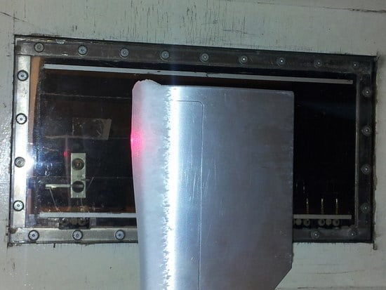
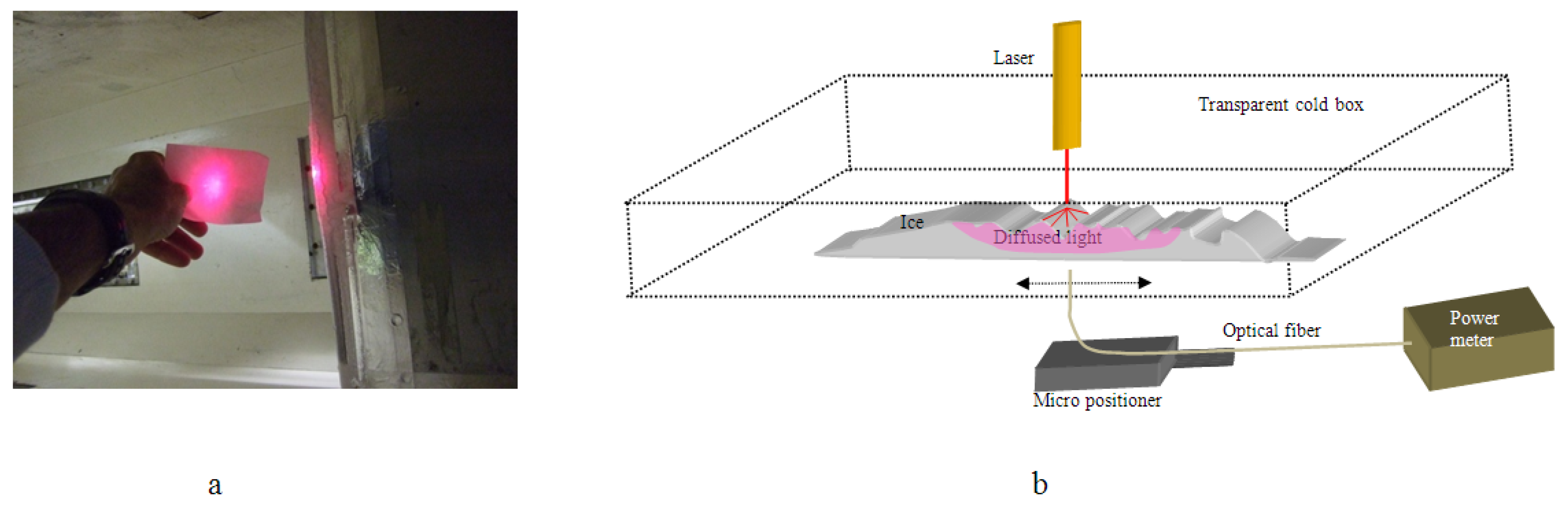
The above experimental results indicate that the optical properties of ice are dependent on the icing conditions, and aerodynamics. These parameters modify the accretion rate, surface and volume morphology of the ice, and are dependent on how rapidly the super-cooled droplets freeze on impact, and hence are directly related to the FF values. For FOAIS, the optical diffusion is a key parameter in identifying ice type; through the relative contributions of the specular reflections and backscattering in the ice growth curves, it is important to investigate the scattering penetration or diffusion in the different types of ice. An example of this is shown in Figure 11a where glazed ice, accepted on the leading edge of the wing, allowed most of the illumination beam to be transmitted, with low scattering contributions. Conversely, in rime ice, light diffuses much further into the ice volume, and the small size of the FOAIS cannot measure the full extent of the optical diffusion. This can be seen in the case of rime ice, Figure 11a,b, where the ice growth curves of the outer fibers give relatively high intensities, indicating that light penetrates deeper in this type of ice.
To investigate, quantitatively, optical diffusion in the different types of ice, sections of ice similar to those shown in Figure 1 were extracted from the wing at the end of icing runs, and stored in a freezer for a short time to preserve their structure while their optical properties were measured off-line. Using the experimental arrangement shown in Figure 11b, ice sections, of about 10 mm thick, were placed in a transparent refrigerated cool-box, and illuminated perpendicularly on the windward surface by a stationary laser beam with a wavelength of 630 nm, and beam diameter of about 2 mm. The beam diffused in the ice, and was detected on the opposite side by an optical fiber mounted on a liner translation micromanipulator, which scanned the flat bottom surface of the ice, measuring the transmitted intensity with an optical power meter. The transmitted intensities for the different types of ice, accreted at temperatures ranging from −10 °C to −20 °C, as a function of distance from the centrally located laser beam (designated as 0 mm), are shown in Figure 12a, and resemble a Gaussian distribution. The optical penetration, in the different types of ice, was measured using the intensity Full-Width-Half-Maxima (FWHM), plotted as a function of temperature, and shown in Figure 12b. For glazed ice which has a low FF value, it shows that the variations of the optical diffusion, accreted at temperatures of −5 °C to −10 °C, have a FWHM of about 3 mm to 3.5 mm. As the FF value of ice progressively increases toward 1, and the ice becomes progressively rime at temperatures from −15 °C to −20 °C, light diffuses over a wider area having a FWHM of 4.1 mm to 7.5 mm. In essence, these results show that the freezing process on the wing, which influences the concentrations of the micro-bubbles in the ice volume, is thus directly related to the way light diffuses in the ice, as shown quantitatively by the FWHM in Figure 12b. This result highlights the close dependence of the FF parameter on the optical diffusion in the different types of ice, and hence on the ice growth curves.
5.4. Freezing Fraction Correlation with Ice Sensor Optical Diffusion
Based on the above experimental results and discussions, it was postulated that the FF can be correlated directly to the optical intensity ice growth curves of the inner fibers shown in Figure 9. As the FF values are representative of the physical process of freezing, it was hypothesized that they may also be related to the concentrations of the micro-bubbles trapped in the ice volume, and thus the optical properties of accreting ice. This hypothesis is based on the observation that when the FF values are low, 0.1 to 0.3 for instance, the freezing process is slow, so the dissolved gasses in the super-cooled droplets can escape accreting glazed transparent ice. Therefore, as discussed earlier for this type of ice, the inner fibers, which detect reflected and scattered light, give a maximum intensity for ice thickness of about 3 to 4 mm of ice. Furthermore, as glazed ice has low concentrations of scatterers, the detected intensity reduces with increasing ice thickness, giving the characteristic ice growth curves shown in Figure 9a.
For FF close to 1, on the other hand, the super-cooled droplets freeze instantaneously trapping the dissolved gasses, forming high densities of micro-bubbles, thus accreting white opaque rime ice. Therefore, the detected light is predominantly due to scattering, with small reflection contributions, as shown in Figure 9c,d. Therefore, based on these observations, a parameterization of the reflection and scattering contributions is postulated, and is in conjunction with modeling of the detection process for the different types of ice, and a semi-empirical correlation of the FF with the optical diffusion is proposed below.
With reference to Figure 9a–d, the ratio of reflected to scattered light, measured by the inner fibers, changes for the different types of ice, and can be used to link these two parameters. The investigation involved calculating the FF values from the icing tunnel experimental parameters, based on Anderson and Tsao’s work [22], and comparing them to the ice growth curves of the two inner fibers, which detected both the reflected and backscattered light. The FF was calculated for steady conditions in the icing tunnel using relation (9) and relation (10), outlined in Section 2.3.3. The values for Ac were calculated using icing tunnel parameters such as the LWC, total ice thickness measured primarily by the FOAIS, as well as shadowgraph and air speed, while the collection efficiency β0 of the airfoil was taken from the NASA Glenn data by virtue of using a near identical wing. It is therefore proposed that the ice growth curves, measured by the
FOAIS for the different types of ice, can be used to characterize quantitatively the ice type by comparing the relative reflection and backscattered contribution to the optical signals, correlating them to corresponding FF values. For this analysis, several ice growth data were taken under identical icing tunnel conditions for glazed, mixed phase, and rime ice. These were subsequently averaged, normalized, and the results for the inner fibers 3 and 4 are shown in Figure 13. It is evident that the ice growth curves can be divided broadly in the region where reflections dominate, giving the distinct intensity peak at around 2 mm to 3 mm of ice thickness with a maximum normalized intensity value, which for convenience was designated as a reflection parameter a, as seen in Figure 13. Similarly, at greater ice thicknesses where scattering predominates, the signals generally level off, having a constant value which can be lower than the reflection peak, as in the case of glazed ice, which increases as the ice becomes progressively rime. Therefore, an equivalent scattering intensity parameter, designated as b, can be measured at the point where the scattering signal is nearly constant i.e., when dI/dx ~ 0, which in Figure 13 is shown at an ice thickness of about 8 mm to 10 mm.
Observing the normalized ice growth curves in Figure 13, the exact values of a and b parameters for the different types of ice are not always clear. The reflection parameter a for glazed and mixed phase ice is quite distinct, whereas the scattering parameter b for these types of ice is not as clear due to the gradient dI/dx not being zero. Specifically, the reflection parameter a, for glazed and mixed phase ice—accreted at −5 °C, −10 °C, −20 °C, and shown in Figure 13 in black, red, and blue, respectively—is quite distinct, and can easily be identified, but it is not the same for the scattering parameter b. The same uncertainty exits for the reflection parameter a for rime ice accreted at −25 °C, as this trace has no distinct reflection value from which it can be measured accurately.
This was resolved by using the simulations for glazed and rime ice, as outlined in Section 4 (Figure 5), to determine the maximum reflected and scattered signals by tailoring the modeling parameters to reproduce the experimental results obtained in Figure 13. Specifically, modeling results for all types of ice, shown in Figure 5, display the reflection and scattering trace in black and red, respectively, with the combined traces being in blue. Thus, for rime ice, the reflection peak, identified from the black trace in Figure 5, designates the reflection parameter a. Similarly, when the reflection and scattering traces intersect the blue trace, dI/dx ~ 0, they designate the scattering parameter b. Based on these assumptions, the modeling and experimental results can be used to identify the points at which a and b can be measured. Furthermore, it transpires that the peak reflections, for all the types of ice, are dependent on the fiber NA and occur at about 2 mm to 3 mm of ice thickness, while the scattering parameter b is measured at about 8 mm to 10 mm of ice.
Based on the above arguments, the relative ratios of the scattering and reflection parameters b/a can be calculated and compared with the corresponding FF values calculated from the icing tunnel parameters, as described previously. These results show that the normalized intensity ratios b/a vary as the ice changes from glazed to rime, with the value of a being larger than b for glazed ice, and gradually becoming equal as the ice becomes rime. There is a caveat, however, in this methodology for the case of rime ice, as the scattering parameter b may, on some occasions, exceed the reflection parameter a, giving values greater than 1. This can be attributed to the FOAIS parameters, and is currently being investigated. However, when that occurs, the ice is totally rime with an FF of 1, and therefore b/a ratio can also be assumed as equal to 1.
In order to investigate the relation of the FF values to the b/a parameter, we initially compare the FF values obtained in the GKN icing tunnel with those of Anderson and Tsao [22] in the NASA Glenn tunnel, using a similar dimension wing. The leading edge of their wing had a diameter d and chord c, of 0.8 cm and 26.7 cm, respectively. The icing condition used in their experiments had airspeeds in the range of 160 knots to 170 knots, with LWC ranging from 1.1 to 1.2 gm/m3, icing runs durations τ of about 2.5 min, and temperatures ranging from −7 °C to −20 °C. The calculated FF values as a function of temperature, using relations (9, 10) from Anderson and Tsao data, are shown in Figure 14 in red, which exhibits a linear relation with a gradient of −0.029 ∓ 0.002/degree C. In our experiments, the FOAIS was mounted on the stagnation line, at the midpoint of the wing as shown in Figure 2b, having a diameter d of 0.89 cm, and a cord of 31 cm. It was positioned in the center of the GKN icing tunnel, which had a width to height cross-section of 76 cm by 51 cm, respectively. The icing conditions used were similar to those of Anderson and Tsao, with airspeed ranging from 150 knots to 165 knots, temperatures from −5 °C to −25 °C, LWC of about 1 gm/m3, and droplet MVD of about 20 μm.
The ice thickness was measured by the calibrated FOAIS, as well as by the shadowgraph for verification purposes. Several experiments were conducted with the same icing conditions and temperatures, with average icing runs τ lasting from 2.5 to 5 min, accreting between 7 mm to 13 mm of ice. As outlined in Section 3, the density of the cloud and LWC was monitored using the forward scattering of the shadowgraph beam as it illuminated the cloud. By scanning the shadowgraph beam along the leading edge of the wing, in the vicinity of the fiber optic ice sensor, it was possible to monitor qualitatively the cloud distribution in the beginning of icing runs. The FF values for our wing were calculated using the same relations (9, 10), and the results are shown in in Figure 14 in the black trace. Similarly to the NASA-Glenn results, this trace is also linear having a gradient of −0.042 ∓ 0.002/degree C. The slight variation in the gradients of the two wings can be attributed to the slightly different characteristics of the icing tunnels, but generally the two results are linear.
Finally, in order to verify the hypothesis that the FF values are correlated to the optical characteristic of ice through the b/a parameters, both b/a, ratios and the FF values were plotted as a function of temperature. Thus, using the normalized ice growth curves obtained from the inner fibers 3, 4 of the array ice sensor, the ratio b/a, obtained from a number of experiments similar to those shown in Figure 13, was plotted as a function of temperature, and the results are shown in the red trace in Figure 15a. As can be seen from this figure, the ratio b/a has values between 0 and 1 just like the FF, and is also linear with temperature having a negative gradient of −0.032 ∓ 0.007/degree C. Furthermore, for comparison, in Figure 15a the black trace is the calculated FF of our wing as a function of temperature, copied from Figure 14. Comparing the gradients of these two traces, it can be seen that their slopes are similar, having values of −0.032 ∓ 0.007/degree C for the b/a ratio, and −0.042 ∓ 0.002/degree C for the calculated FF. There two traces indicate a strong correlation between the two parameters which can be seen more clearly if the ratio b/a and the FF values are plotted together, i.e., the two traces in Figure 14 are plotted in Figure 15b. It is apparent that there is a close correlation of the two parameters, exhibiting a linear relation with a gradient of about 0.75. This indicates the value of our assumption that the ice growth curves through the relative contributions from the reflected and scattered intensities, i.e., the parameter b/a, can be correlated directly to the FF of the wing in the icing tunnel.
This is the proof-of-concept semi-empirical verification of the correlation of the FF with the b/a ratio, enabling the FOAIS to be used initially as a research tool in the development of aircraft wings to determine both the ice thickness type, as well as the FF of the accreting ice. Furthermore, it has the potential to be used in real time on wings to measure the ice thickness through suitable calibration using the shadowgraph technique, as well as to identify the ice type and its FF, provided that the wing can accept a maximum ice thickness of 10 mm. This is acceptable if the FOAIS is located on the inner thicker sections of the wing where ice tolerances are greater due to the large leading-edge diameter. The significance of this sensor is that it gives quantitative information on the type of ice accreted on the wings of the aircraft, through the b/a ratio, and on ice severity conditions which can potentially include SLD ice. Furthermore, the FOAIS potentially has the ability to measure the onset of icing, with thicknesses ranging from almost 0.1 mm of ice to about 10 mm using the inner and outer fiber. Additionally, it permits a number of alternative de-ice strategies which include allowing the ice to reach a certain thickness prior to de-icing so the ice will shed-off rather than melt, thus reducing secondary icing further back on the wing, as well as reducing power consumption. An additional potential benefit is that by knowing the ice thickness and the type of ice, the de-icing heater sequencing can be tailored appropriately, thus reducing power requirements.
6. Conclusions
In this work, we used an optical FOAIS, located on the leading edge of a wing in an icing tunnel, to investigate experimentally the optical and diffusion properties of light in the different types of ice accreted, and calibrated it with a shadowgraph technique to measure the ice thickness and type. By modeling the reflection and scattering intensities of the light coupled in the FOAIS as a function of ice thickness, we were able to reproduce the experimental results for the different types of ice accreted on the stagnation line of the wing. Furthermore, using published data from the NASA-Glenn FF studies, we calculated the FF values for a wing in GKN research icing tunnel and demonstrated, as proof-of-concept, the correlation of the FF to the optical diffusion of light in ice by using the normalized ratio of the scattered and reflected intensities detected by the fiber array, b/a parameter. Based on the icing tunnel experimental results and using a shadowgraph technique, it was possible to measure up to 10 mm of ice thickness, with an accuracy of about to 0.5 mm, by utilizing a combination of the inner and outer fibers. However, more work needs to be done to improve these measurements for different types of ice. Furthermore, the type of ice could be determined and correlated to the FF by its optical diffusion though its scattering and reflection characteristics, namely parameters b/a. If the sensor can be located in a section of the wing which can tolerate ice thicknesses of about 10 mm, the system can be used on wings of an aircraft to measure, in real time, the FF which is significant. This, thus, bridges the gap between the two different schools of thought in ice detection/protection. Additionally, by categorizing the type of ice through its FF value, it can be used to potentially identify ice severity, and to optimize the de-icing process. However, more work needs to be done to further validate this proof-of-concept, expanding it to more variables such as LWC, MVD, different types of wings, and temperatures.
Funding
This work was undertaken partly under the ON-WINGS EU projects (FP7-AAT-2008-RTD-1).
Data Availability Statement
Not applicable.
Acknowledgments
I would like to thank Ian Stott, David Armstrong, and Glenn Howards, from GKN aerospace, Nikolaos Kourkoumelis from the University of Ioannina, and Dimitris Syvridis from the University of Athens for their very helpful discussions.
Conflicts of Interest
The author declare no conflict of interest.
References
- Natinal Transportation Safety board Aircraft Accident Report, ATR Model 72–212, Roselawn Indiana, 31 October 1994, NTSB/AAR-6/01. 1996, Volume 1. Available online: https://libraryonline.erau.edu/online-full-text/ntsb/aircraft-accident-reports/AAR96-01.pdf (accessed on 23 October 2022).
- Lynch, F.T.; Khodadoust, A. Effects of ice accretions on aircraft aerodynamics. Prog. Aerosp. Sci. 2001, 37, 669–767. [Google Scholar] [CrossRef]
- Jackson, D.G.; Goldberg, J.I. Ice Detection Systems: A Historical Perspective. In Proceedings of the 2007 SAE Aircraft & Engine Icing International Conference, Seville, Spain, 24–27 September 2007. SAE Technical Paper. [Google Scholar]
- Keith, W.D.; Mill, C.S.; Saunders, C.P.R. A hot-wire instrument to measure liquid water content for use in the laboratory. J. Phys. E Sci. Instrum. 1986, 19, 436–437. [Google Scholar] [CrossRef]
- Umair Najeeb Mughal, Muhammad Shakeel Virk, Atmospheric Icing Sensors—An Insight. In Proceedings of the SENSORCOMM 2013: The Seventh International Conference on Sensor Technologies and Applications, Barcelona, Spain, 25–31 August 2013; pp. 191–199, ISBN 978-1-61208-296-7.
- Melody, W.; Basar, T.; Perkins, W.R.; Voulgaris, P.G. Parameter identification for inflight detection and characterization of aircraft icing. Control Eng. Pract. 2000, 8, 985–1001. [Google Scholar] [CrossRef]
- Haggerty, J.; Defer, E.; De Laat, A.; Bedka, K.; Moisselin, J.; Potts, R.; Delanoë, J.; Parol, F.; Grandin, A.; Divito, S. Detecting clouds associated with jet engine ice crystal icing. Bull. Am. Meteorol. Soc. 2019, 100, 31–40. [Google Scholar] [CrossRef] [PubMed]
- Mason, J.; Strapp, W.; Chow, P. The Ice Particle Threat to Engines in Flight. In Proceedings of the 44th AIAA Aerospace Sciences Meeting and Exhibit, Reno, NV, USA, 9–12 January 2006. [Google Scholar]
- Addy, H.E., Jr.; Veres, J.P. An Overview of NASA Engine Ice-Crystal Icing Research. In Proceedings of the International Conference on Aircraft and Engine Icing and Ground Deicing, Chicago, IL, USA, 13–17 June 2011. NASA/TM—2011-217254. [Google Scholar]
- Roy, S.; Izad, A.; DeAnna, R.G.; Mehregany, M. Smart ice detection system based on resonant piezoelectric transducer. Sens. Actuators A 1998, 69, 243–250. [Google Scholar] [CrossRef]
- DeAnna, R.G.; Mehregany, M.; Roy, S. Micro fabricated ice-detection sensor. In Proceedings of the Smart Structures and Materials Conference, San Diego, CA, USA, 2–6 March 1997; NASA TM-107432. pp. 1–10. [Google Scholar]
- Vellekoop, M.J.; Jakoby, B.; Bastemeijer, J. A Love-Wave Ice Detector. In Proceedings of the 1999 IEEE Ultrasonics Symposium, Tahoe, NV, USA, 17–20 October 1999; pp. 453–456, ISBN 0-7803-5722-1. [Google Scholar]
- Kozak, R.; Wiltshire, B.D.; Khandoker, M.A.R.; Golovin, K.; Zarifi, M.H. Modified microwave sensor with a patterned ground heater for detection and prevention of ice accumulation. ACS Appl. Mater. Interfaces 2020, 12, 55483–55492. [Google Scholar] [CrossRef] [PubMed]
- Wiltshire, B.; Mirshahidi, K.; Golovin, K.; Zarifi, M.H. Robust and sensitive frost and ice detection via planar microwave resonator sensor. Sens. Actuators B Chem. 2019, 301, 126881. [Google Scholar] [CrossRef]
- Schlegl, T.; Moser, M.; Loss, T.; Unger, T. A Smart Icing Detection System for Any Location on the Outer Aircraft Surface. In Proceedings of the International Conference on Icing of Aircraft, Engines, and Structures, Minneapolis, MN, USA, 17–21 June 2019. SAE Technical Paper 2019-01-1931. [Google Scholar] [CrossRef]
- McCann, D.W. NNICE—A neural network aircraft icing algorithm. Environ. Model. Softw. 2005, 20, 1335–1342. [Google Scholar] [CrossRef]
- Ikiades, A. Direct ice detection based on fiber optic sensor architecture. Appl. Phys. Lett. 2007, 91, 104104-1–104104-3. [Google Scholar] [CrossRef]
- Ge, J.; Ye, L.; Zou, J. A novel fiber-optic ice sensor capable of identifying ice type accurately. Sens. Actuators A 2012, 175, 35–42. [Google Scholar] [CrossRef]
- González del Val, M.; Mora Nogués, J.; García Gallego, P.; Frövel, M. Icing Condition Predictions Using FBGS. Sensors 2021, 21, 6053. [Google Scholar] [CrossRef] [PubMed]
- Messinger, B.L. Equilibrium Temperature of an Unheated Icing Surface as a Function of Airspeed. J. Aeron. Sci. 1953, 20, 29–42. [Google Scholar] [CrossRef]
- Petrenko, V.F.; Whitworth, R.W. Physics of Ice; Oxford University Press: Oxford, UK, 2003; pp. 256–270. [Google Scholar]
- Anderson, D.N.; Tsao, J.C. Evaluation and Validation of the Messinger Freezing Fraction. In Proceedings of the 41st Aerospace Sciences Meeting and Exhibit, Reno, NV, USA, 6–9 January 2003; National Aeronautics and Space Administration Glenn Research Center: Cleveland, OH, USA, 2005. NASA/CR-2005-213852, AIAA-2003-1218. [Google Scholar] [CrossRef] [Green Version]
- Zuev, V.E.; Kabanov, M.V.; Savelev, B.A. Propagation of Laser Beams in Scattering Media. Appl. Opt. 1969, 8, 137–141. [Google Scholar] [CrossRef] [PubMed]
- Jacques, S.L. Optical properties of biological tissues. Phys. Med. Biol. 2013, 58, 5007–5008. [Google Scholar] [CrossRef]
Figure 1.
Pictures of ice, accreted on the leading edge of the wings and cross-sections, (a,b) glaze ice accreted at −3 °C (c,d) mixed phase ice accreted at −7 °C to −13 °C (e,f), rime ice accreted at −20 °C and below.
Figure 1.
Pictures of ice, accreted on the leading edge of the wings and cross-sections, (a,b) glaze ice accreted at −3 °C (c,d) mixed phase ice accreted at −7 °C to −13 °C (e,f), rime ice accreted at −20 °C and below.

Figure 2.
(a) Schematic diagram of Fiber optics array ice sensor (FOAIS). (b) Picture of the sensor. (c) Ice sensor on leading edge of the wing with window.
Figure 2.
(a) Schematic diagram of Fiber optics array ice sensor (FOAIS). (b) Picture of the sensor. (c) Ice sensor on leading edge of the wing with window.

Figure 3.
(a) Schematic diagram of reflected and backscattered light from the ice–air interface which falls within the acceptance angle of the signal fibers. (b) Backscattered light which is detected by the signal fibers.
Figure 3.
(a) Schematic diagram of reflected and backscattered light from the ice–air interface which falls within the acceptance angle of the signal fibers. (b) Backscattered light which is detected by the signal fibers.

Figure 4.
(a) Schematic diagram of experimental set up in icing tunnel. (b) Wing with ice in icing tunnel. (c) Shadowgraph beam in icing tunnel.
Figure 4.
(a) Schematic diagram of experimental set up in icing tunnel. (b) Wing with ice in icing tunnel. (c) Shadowgraph beam in icing tunnel.

Figure 5.
Modeling of the reflections (black), scattering (red), and combined reflection and scattering (blue) contributions to the optical signal detected by the fiber 4 (next to the source fiber) for (a) glazed ice, (b) mixed phase ice, (c) and rime ice.
Figure 5.
Modeling of the reflections (black), scattering (red), and combined reflection and scattering (blue) contributions to the optical signal detected by the fiber 4 (next to the source fiber) for (a) glazed ice, (b) mixed phase ice, (c) and rime ice.

Figure 6.
Simulation of the total optical intensities detected by fibers 4, 5, 6, on one side of the source fiber: (a) glazed ice, (b) for near rime ice.
Figure 6.
Simulation of the total optical intensities detected by fibers 4, 5, 6, on one side of the source fiber: (a) glazed ice, (b) for near rime ice.

Figure 7.
Shadowgraph calibration. The black trace shows the beam blockage, and the red trace is for convenience I = (I0 − Ix).
Figure 7.
Shadowgraph calibration. The black trace shows the beam blockage, and the red trace is for convenience I = (I0 − Ix).

Figure 8.
(a) Typical ice growth curves obtained by the fiber array ice sensor for glazed ice accreted at −5 °C to −7 °C. (b) Pictures from a typical icing tunnel run showing ice accession together with the corresponding signals of the ice sensor during ice growth.
Figure 8.
(a) Typical ice growth curves obtained by the fiber array ice sensor for glazed ice accreted at −5 °C to −7 °C. (b) Pictures from a typical icing tunnel run showing ice accession together with the corresponding signals of the ice sensor during ice growth.

Figure 9.
Comparative ice growth curves from the fiber array ice sensor (a), glazed ice accreted at −5 °C to −7 °C (b), for mixed phase ice accreted at −10 °C to −15 °C (c), nearly rime ice accreted at −20 °C (d), and totally rime ice accreted at −25 °C.
Figure 9.
Comparative ice growth curves from the fiber array ice sensor (a), glazed ice accreted at −5 °C to −7 °C (b), for mixed phase ice accreted at −10 °C to −15 °C (c), nearly rime ice accreted at −20 °C (d), and totally rime ice accreted at −25 °C.

Figure 10.
(a) Ice growth curves for fibers 4, 5, 6 together with shadowgraph tailored for fiber 5; (b) shadowgraph calibration curve for inner fiber 4 and outer fiber 6 with shadowgraph tailored for fiber 6.
Figure 10.
(a) Ice growth curves for fibers 4, 5, 6 together with shadowgraph tailored for fiber 5; (b) shadowgraph calibration curve for inner fiber 4 and outer fiber 6 with shadowgraph tailored for fiber 6.

Figure 11.
(a) Illumination through ice from inside the wing. (b) Schematic diagram of optical diffusion experimental set up using section of ice, taken at the end of icing runs, and measured in a cool box.
Figure 11.
(a) Illumination through ice from inside the wing. (b) Schematic diagram of optical diffusion experimental set up using section of ice, taken at the end of icing runs, and measured in a cool box.

Figure 12.
(a) Optical diffusion of a laser beam, measured as the transmitted intensity distribution as a function of distance in mm, for ice accreted at different temperatures. (b) Optical diffusion measured in mm, manifested as the FWHM of the transmitted intensities through ice accreted at different temperatures.

Figure 13.
Typical normalized ice growth curves of the inner signal fiber 4 obtained at temperatures of −5 °C to −25 °C.
Figure 13.
Typical normalized ice growth curves of the inner signal fiber 4 obtained at temperatures of −5 °C to −25 °C.

Figure 14.
Comparison of icing tunnel calculated FF using Messinger’s relation [20], for wing in NASA Glenn icing tunnel (red), and FF for wing incorporating the fiber array ice sensors in GKN icing tunnel (black).
Figure 14.
Comparison of icing tunnel calculated FF using Messinger’s relation [20], for wing in NASA Glenn icing tunnel (red), and FF for wing incorporating the fiber array ice sensors in GKN icing tunnel (black).

Figure 15.
Comparison of b/a parameter with FF: (a) Scattering and reflection intensities ratio b/a parameter as a function of temperature, (red trace), and calculated FF of the wing in the icing tunnel (repeated trace taken from Figure 13). (b) Correlation of FF of our wing in icing tunnel, with the b/a parameter.

Disclaimer/Publisher’s Note: The statements, opinions and data contained in all publications are solely those of the individual author(s) and contributor(s) and not of MDPI and/or the editor(s). MDPI and/or the editor(s) disclaim responsibility for any injury to people or property resulting from any ideas, methods, instructions or products referred to in the content. |
© 2022 by the author. Licensee MDPI, Basel, Switzerland. This article is an open access article distributed under the terms and conditions of the Creative Commons Attribution (CC BY) license (https://creativecommons.org/licenses/by/4.0/).
Share and Cite
MDPI and ACS Style
Ikiades, A. Fiber Optic Ice Sensor for Measuring Ice Thickness, Type and the Freezing Fraction on Aircraft Wings. Aerospace 2023, 10, 31. https://doi.org/10.3390/aerospace10010031
AMA Style
Ikiades A. Fiber Optic Ice Sensor for Measuring Ice Thickness, Type and the Freezing Fraction on Aircraft Wings. Aerospace. 2023; 10(1):31. https://doi.org/10.3390/aerospace10010031
Chicago/Turabian StyleIkiades, Aris. 2023. "Fiber Optic Ice Sensor for Measuring Ice Thickness, Type and the Freezing Fraction on Aircraft Wings" Aerospace 10, no. 1: 31. https://doi.org/10.3390/aerospace10010031
Note that from the first issue of 2016, this journal uses article numbers instead of page numbers. See further details here.